CODE:
Get the code used for this section here
Using digital soil mapping to update, harmonize and disaggregate legacy soil maps.
Pre-reading background
Digital soil maps are contrasted from legacy soil maps mainly in terms of the underlying spatial data model. Digital soil maps are based on the pixel data model, while legacy soil maps will typically consist of a tessellation of polygons.
The advantage of the pixel model is that the information is spatially explicit. The soil map polygons are delineations of soil mapping units which consist of a defined assemblage of soil classes assumed to exist in more-or-less fixed proportions. There is great value in legacy soil mapping because a huge amount of expertise and resources went into their creation.
Digital soil mapping will be the richer by using this existing knowledge-base to derive detailed and high resolution digital soil products. However the digitization of legacy soil maps is not digital soil mapping. Rather, the incorporation of legacy soil maps into a digital soil mapping workflow involves some method (usually quantitative) of data mining, to appoint spatially explicit soil information — usually a soil class or even a measurable soil attribute — upon a grid the covers the extent of the existing (legacy) mapping.
In some ways, this process is akin to downscaling because there is a need to extract soil class or attribute information from aggregated soil mapping units. A better term therefore is soil map disaggregation.
There is an underlying spatial explicitness in digital soil mapping that makes it a powerful medium to portray spatial information. Legacy soil maps also have an underlying spatial model in terms of the delineation of geographical space. However, there is often some subjectivity in the actual arrangement and final shapes of the mapping unit polygons. Yet that is a matter of discussion for another time.
For disaggregation studies the biggest impediment to overcome in a quantitative manner is to determine the spatial configuration of the soil classes within each map unit. It is often known which soil classes are in each mapping unit, and sometimes there is information regarding the relative proportions of each too. What is unknown is the spatial explicitness and configuration of said soil classes within the unit. This is the common issue faced in studies seeking the renewal and updating of legacy soil mapping.
Some examples of soil map disaggregation studies from the literature include Thompson et al. (2010) who recovered soil-landscape rules from a soil map report in order to map individual soil classes. This together with a supervised classification approach described by Nauman et al. (2012) represent manually-based approaches to soil map disaggregation. Both of these studies were successfully applied, but because of their manual nature, could also be seen as time-inefficient and susceptible to subjectivity.
The flip side to these studies is those using quantitative models. Usually the modeling involves some form of data mining algorithm where knowledge is learned and subsequently optimized based on some model error minimization criteria. Extrapolation of the fitted model is then executed in order to map the disaggregated soil mapping units. Such model-based or data mining procedures for soil map disaggregation include that by Bui and Moran (2001) in Australia, Haring et al. (2012) in Germany and Nauman and Thompson (2014) in the USA. Some fundamental ideas of soil map disaggregation framed in a deeper discussion of scaling of soil information are presented in McBratney (1998).
This section seeks to describe a soil map disaggregation method that was first described in Wei et al. (2010) for digital harmonization of adjacent soil surveys in southern Iowa, USA. The concept of harmonization has particular relevance in the USA because it has been long established that the underlying soil mapping concepts across geopolitical boundaries (i.e. counties and states) don’t always match. This issue is obviously not a phenomenon exclusive to the USA but is a common worldwide issue. This mismatch may include the line drawings and named map units. Of course, soils in the field do not change at these political boundaries. These soil-to-soil mismatches are the result of the past structuring of the soil survey program. For example, soil surveys in the US were conducted on a soil survey area basis. Most times the soil surveys areas were based on county boundaries. Often adjacent counties were mapped years apart. Different personnel, different philosophies of soil survey science, new concepts of mapping and the availability of various technologies all have played a part in why these differences occur. These differences maybe even more exaggerated at state lines as each state was administratively and technically responsible for the soil survey program within a given state.
The algorithm developed by Wei et al. (2010) addressed this issue, where soil mapping units were disaggregated into soil series. Instead of mapping the prediction of a single soil series, a probability distribution of all potential soil series was estimated. The outcome of this was the dual disaggregation and harmonization of existing legacy soil information into raster-based digital soil mapping product/s.
Odgers et al. (2014) using legacy soil mapping from an area in Queensland, Australia refined the algorithm to which they called DSMART or, Disaggregation and Harmonization of Soil Map Units Through Re-sampled Classification Trees*.
Besides the work of Odgers et al. (2014), The DSMART algorithm has been used in other projects throughout the world, with Chaney et al. (2014) using it to disaggregate the entire gridded USA Soil Survey Geographic (gSSURGO) database. The resulting POLARIS data set (Probabilistic Remapping of SSURGO) provides the 50 most probable soil series predictions at each 30-meter grid cell over the contiguous USA.
The DSMART algorithm has been pivotal, together with the associated PROPR algorithm (Digital Soil Property Mapping Using Soil Class Probability Rasters (Odgers et al. (2015)) in deriving high resolution digital soil maps where point-based DSM approaches cannot be undertaken, particularly where soil point data is sparse.
DSMART: an overview
Odgers et al. (2014) provide a detailed explanation of the DSMART algorithm. The aim of DSMART is to predict the spatial distribution of soil classes by disaggregating the soil map units of a soil polygon map. Here soil map units soil map are entities consisting of a defined set of soil classes which occur together in a certain spatial pattern and in an assumed set of proportions.
The DSMART method of representing the disaggregated soil class distribution is as a set of numerical raster surfaces, with one raster per soil class. The data representation for each soil class is given as the probability of occurrence. In order to generate the probability surfaces, a re-sampling approach is used to generate n realizations of the potential soil class distribution within each map unit. Then at each grid cell, the probability of occurrence of each soil class is estimated by the proportion of times the grid cell is predicted as each soil class across the set of realizations.
The procedure of the DSMART algorithm can be summarized in 6 main steps:
- Draw n random samples from each soil map polygon. This could be the same number of samples per polygon or area weighted.
-
Assign soil class to each sampling point.
- Weighted random allocation from soil classes in relevant map unit
- Relative proportions of soil classes within map units are used as the weights
- Use sampling points and intersected covariate values to build a decision tree to prediction spatial distribution of soil classes.
- Apply decision tree across mapping extent using covariate layers.
- Steps 1-4 repeated i times to produce i realizations of soil class distribution.
- Using i realizations generate probability surfaces for each soil class.
The model type that Odgers et al. (2014) used was the C4.5 decision tree algorithm which was developed by Quinlan (1993). The type of data mining algorithm implemented in DSMART is not prescriptive; as long as it is robust and importantly, computationally efficient. For example Chaney et al. (2014) used Random Forest models Breiman (2001) in their own implementation.
Implementation of DSMART
The DSMART algorithm has previously been written in the C++ and
Python computing languages. It is also available in an R package.
Regardless of computing language preference, DSMART requires three chief
sources of data
- The soil map unit polygons that will be disaggregated.
- Information about the soil class composition of the soil map unit polygons.
- Geo-referenced raster covariates representing the scorpan factors of which have complete and continuous coverage of the mapping extent. There is no restriction in terms of the data type i.e. continuous, categorical, ordinal etc.
The DSMART algorithm is packaged up in rdsmart and contains two
working functions: disaggregate and summarise. More will be
discussed about these shortly.
The other items in the package are various inputs required to run the function. In essence these data provide some indication of the structure and nature of the information that is required to run the DSMART algorithm so that it can be easily adapted to other projects.
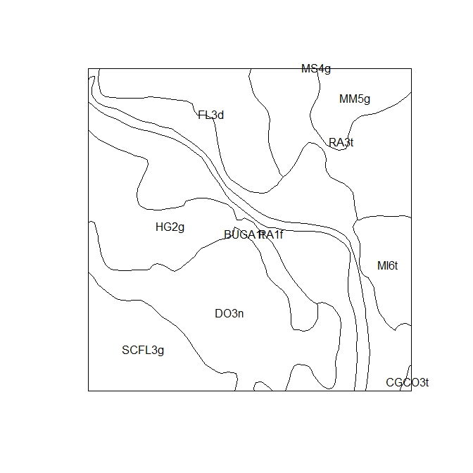
First is the soil map to be disaggregated. This is saved to the
dalrymple_polygons object. In this example the small polygon map is a
clipped area of the much larger soil map that Odgers et al. (2014)
disaggregated, which was the 1:250,000 soil map of the Dalrymple Shire
in Queensland Australia by Rogers, Cannon, and Barry (1999).
In this example data set, there are 11 soil mapping units.the polygon
object is of class SpatialPolygonsDataFrame, which is what would be
created if you were to read in a shapefile of the polygons into R.
# install rdsmart library(devtools)
# devtools::install_bitbucket('brendo1001/dsmart')
library(rdsmart)
library(sf)
library(terra)
library(sp)
library(raster)
# Note rdsmart is yet to migrate functionality to the sf and terra
# R packages, there the example currently runs using the now legacy
# sp and raster R packages.

# Polygons
data("dalrymple_polygons")
class(dalrymple_polygons)

## [1] "SpatialPolygonsDataFrame"
## attr(,"package")
## [1] "sp"

summary(dalrymple_polygons$MAP_CODE)

## BUGA1t CGCO3t   DO3n   FL3d   HG2g   MI6t   MM5g   MS4g   PA1f
##      1      1      1      1      1      1      1      1      1
##   RA3t SCFL3g
##      1      1

## Plot polygons
plot(dalrymple_polygons)
invisible(text(getSpPPolygonsLabptSlots(dalrymple_polygons), labels = as.character(dalrymple_polygons$MAP_CODE), cex = 0.8))
The next inputs are the soil map unit compositions which is saved to the
dalrymple_composition object. This is a data.frame that simply
indicates in respective columns the map unit name, and corresponding
numerical identifier label. Then there is the soil classes that are
contained in the respective mapping unit, followed by the relative
proportion that each soil class contributes to the map unit. The
relative proportions will and probably should sum to 100.
# Map unit compositions
data("dalrymple_composition")
head(dalrymple_composition)

##   poly mapunit soil_class proportion
## 1  304    MM5g         RA         70
## 2  304    MM5g         EW         20
## 3  304    MM5g         PI         10
## 4  440  CGCO3t         CG         50
## 5  440  CGCO3t         CO         20
## 6  440  CGCO3t         DA         10
The last required inputs are the environmental covariates. This use used
to inform the model fitting for each DSMART iteration, and ultimately be
used for the spatial mapping. There are actually 20 different covariate
rasters of which have been derived from a digital elevation model and
gamma radiometric data. These rasters are organized into a RasterStack
and are of 30m grid resolution.
data("dalrymple_covariates")
class(dalrymple_covariates)

## [1] "RasterStack"
## attr(,"package")
## [1] "raster"

raster::nlayers(dalrymple_covariates)

## [1] 20

raster::res(dalrymple_covariates)

## [1] 30 30
Now it is time to run the DSMART algorithm. The implementation is spread
across two companion functions already mentioned: disaggregate and
summarise. The disaggregate function is the workhorse of the two
because it performs the sample/resampling, model fitting and iteration
parts of DSMART.
The summarise function works on the outputs of disaggregate to
estimate the probabilities of classes, and derives some other useful
outputs such as the most probable soil class and or n-most probable
soil classes.
Using the disaggregate function, we provide it with the inputs
described above. Additional inputs include the parameters rate, which
is a numeric value for the number of samples to take from each soil
mapping polygon; reals is the number of model realizations to fit; and
cpus is the number of compute nodes to use for the analysis. The
default is to run the algorithm in sequential mode, however it does have
the capability to be scaled up substantially in parallel mode, which
helps to eliminate some computation time.
In the example below we set rate to 15, reals to 10, and cpus
to 1. An unusual yet helpful feature of this function is that none of
the output is saved to the R memory, but instead, directly to file, or
specifically the current working directory into a folder called
outputs.
After the disaggregate function has terminated, you will find in the
outputs folder a few other folders which contain rasters of the soil
class prediction from each iteration. You will also encounter another
folder contain text file outputs from each iteration of the C5 model
structure plus information on the quality of the fit.
test.dsmart <- rdsmart::disaggregate(
covariates = dalrymple_covariates,
polygons = dalrymple_polygons,
composition = dalrymple_composition,
rate = 15, reals = 10, cpus = 1, outputdir = getwd())
The disaggregate function has some added functionality that is not
used in the above example. The help file for the function describes the
added functionality which includes the allowance of observed data into
the algorithm through the observations parameter. The is also
provision of different methods for sampling polygons. There is also an
ability to include additional environmental variables by way of strata
which constrains the occurrences of soil classes to certain areas and or
positions within the landscape.
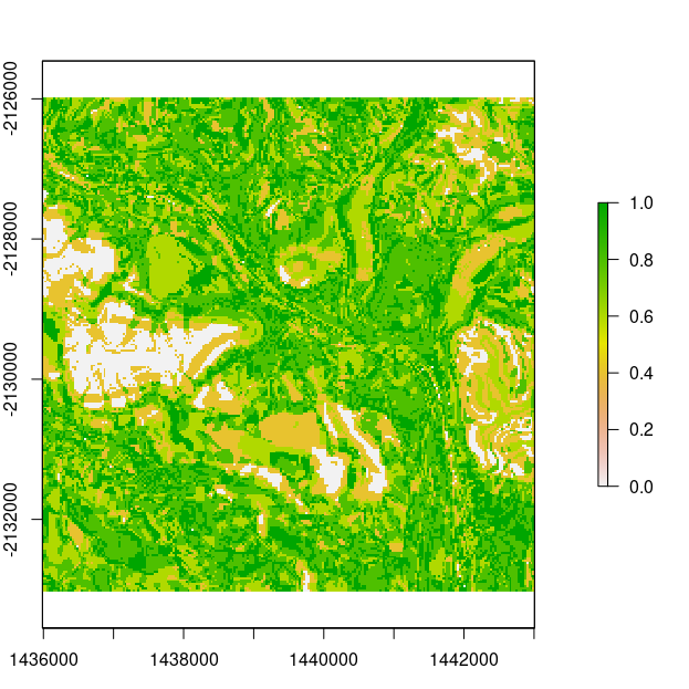
Of particular interest is to derive the soil class probabilities, and even the most probable soil class at each pixel, and even an estimate of the uncertainty, which is given in terms of the confusion index that was used earlier during the fuzzy classification of data for derivation of digital soil map uncertainties.
The confusion index essentially measure how similar to classification is between (in most cases) most probable and second-most probable soil class predictions at a pixel.
To derive the probability rasters we need the rasters that were
generated from the disaggregate function. This can be done via the use
of the list.files function and the raster package to read in the
rasters and stack them into a rasterStack.
Rather than doing this we can use pre-prepared outputs namely in the
form of the dalrymple_realisations (raster outputs from
disaggregate) and dalrymple_lookup (lookup table of soil class names
and numeric counterparts which is an output from disaggregate)
objects. As with disaggregate, summarise can be run in parallel mode
via control of the cpus variable.
The n-most probable rasters are also created by summarise, and are
important for the follow on procedure of soil attribute mapping, of
which is the focus of the study by Odgers et al (2015)
and integral to the associated PROPR algorithm.
In many cases the user may just be interested in deriving the most
probable soil class, or sometimes the n-most probable soil class maps.
The nprob parameter provides user control on the number of
n-probable outputs.
# load pre existing outputs
data(dalrymple_lookup)
data(dalrymple_realisations)

# run summarise function
test.dsmart_summ <- summarise(realisations = dalrymple_realisations, lookup = dalrymple_lookup, nprob = 3, cpus = 1)
A few folders are automatically generated to the working directory which
contain various outputs from the summarise function. These are:
mostprobable and probabilities. The folder mostprobable contains
the n-most probable soil class maps. The folder: probabilities
contains the probability rasters for each candidate soil class.
A confusion index (Burrough et al. 1997) raster may also be returned using the post processing confusion_index function on the stack of the probability rasters that are returned from the summarise function.
Finally lets produce a map of the most probable soil class and the associated map of the confusion index.
## calculate confusion index find the probability rasters
in.dir <- "SOME_DIRECTORY"
prob.files <- list.files(path = paste0(in.dir, "output/probabilities/"), pattern = ".tif", full.names = T, recursive = F)
# stack
prob.rasters <- raster::stack(prob.files)
conf.ind <- rdsmart::confusion_index(prob.rasters, cpus = 1)
plot(conf.ind)
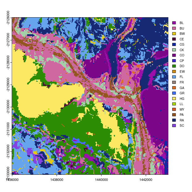
# plot most probable soil class
ml.map <- terra::rast(paste0(in.dir, "output/mostprobable/mostprob_01_class.tif"))
ml.map <- as.factor(ml.map)
# some classes have been dropped from map
levels(ml.map)[[1]][, 1]
# find which ones have not been dropped
rms <- which(test.lookup[, 2] %in% levels(ml.map)[[1]][, 1])
# new look up table for plotting
new.lookup <- test.lookup[rms, ]
levels(ml.map) = data.frame(value = new.lookup[, 2], desc = new.lookup[, 1])
# Randomly selected HEX colors
area_colors <- c("#9a10a8", "#cf68a0", "#e7cc15", "#4f043a", "#1129a3", "#a2d0a7", "#7b0687", "#3e28d1", "#2c8c04", "#d39014", "#66a5ed", "#978279", "#db6f1f", "#4070fc", "#fde864", "#acdb0a", "#d95a28", "#94561f", "#162972", "#8342e1")
# plot
terra::plot(ml.map, col = area_colors, plg = list(legend = new.lookup[, 1], cex = 0.8))
DSMART can be quite a powerful algorithm for disaggregating legacy soil
mapping as demonstrated by Chaney et al. (2014) in the USA. While the
computational effort to generate disaggregated predictions could be a
burden, the DSMART algorithm is relatively easy to parallelize, which
was also demonstrated in Chaney et al. (2014), and with the
implementation of the current R version of this algorithm.
One other restrictive feature of the DSMART algorithm is the need for specific inputs, particularly in regards to the soil class compositions and their relative proportions within mapping units. Sometimes this information is not easily available, and needs to be approximated by some means.
Besides to advantage of generating detailed maps of soil classes, which will have their own use for some applications, the DSMART algorithm provides a pathway to first update and harmonize legacy soil maps, and then to realize soil property information from existing polygon soil maps, such as through the use and coupling of soil class probability rasters and modal soil class profiles as demonstrated in Odgers, McBratney, and Minasny (2015). It is this detailed soil attribute information that is required in land system modeling frameworks, and for ongoing assessment and monitoring of the soil resource.
References
Breiman, L. 2001. “Random Forests.” Machine Learning 41: 5–32.
Bui, E. N., and C. J. Moran. 2001. “Disaggregation of Polygons of Surficial Geology and Soil Maps Using Spatial Modelling and Legacy Data.” Geoderma 103: 79–94. https://doi.org/http://dx.doi.org/10.1016/S0016-7061(01)00070-2.
Burrough, P. A, P. F. M van Gaans, and R Hootsmans. 1997. “Continuous Classifcation in Soil Survey: Spatial Correlation, Confusion and Boundaries.” Geoderma 77: 115–35.
Chaney, Nathaniel, Jonathan W. Hempel, Nathan P. Odgers, Alex B. McBratney, and Eric F. Wood. 2014. “Spatial Disaggregation and Harmonization of gSSURGO.” Long Beach, CA: ASA, CSSA; SSSA.
Haring, T., E. Dietz, S. Osenstetter, T. Koschitzki, and B. Schroder. 2012. “Spatial Disaggregation of Complex Soil Map Units: A Decision-Tree Based Approach in Bavarian Forest Soils.” Geoderma Geoderma 185?186, 37?47.: 37–47. https://doi.org/http://dx.doi.org/10.1016/j.geoderma.2012.04.001.
McBratney, Alex.B. 1998. “Some Considerations on Methods for Spatially Aggregating and Disaggregating Soil Information.” In Soil and Water Quality at Different Scales, edited by PeterA. Finke, Johan Bouma, and MarcelR. Hoosbeek, 80:51–62. Developments in Plant and Soil Sciences. Springer Netherlands. https://doi.org/10.1007/978-94-017-3021-1_5.
Nauman, T W, J A Thompson, N P Odgers, and Z Libohova. 2012. “Digital Soil Assessments and Beyond: Proceedings of the Fifth Global Workshop on Digital Soil Mapping.” In, edited by B Minasny, B. P Malone, and A B McBratney, 203–7. CRC Press, London, UK.
Nauman, Travis W., and James A. Thompson. 2014. “Semi-Automated Disaggregation of Conventional Soil Maps Using Knowledge Driven Data Mining and Classification Trees.” Geoderma 213: 385–99. https://doi.org/http://dx.doi.org/10.1016/j.geoderma.2013.08.024.
Odgers, N P, A B McBratney, and B Minasny. 2015. “Digital Soil Property Mapping and Uncertainty Estimation Using Soil Class Probability Rasters.” Geoderma 237-238: 190–98.
Odgers, N P, W Sun, A B McBratney, B Minasny, and D Clifford. 2014. “Disaggregating and Harmonising Soil Map Units Through Resampled Classification Trees.” Geoderma 214-215: 91–100.
Quinlan, J R. 1993. C4.5: Programs for Machine Learning. Morgan Kaufmann, San Mateo, California.
Rogers, L. G., M. G. Cannon, and E. V. Barry. 1999. Land Resources of the Dalrymple Shire, 1. Land Resources Bulletin DNRQ980090. Brisbane, Australia: Queensland Department of Natural Resources.
Thompson, J A, T Prescott, A C Moore, J Bell, D R Kautz, J W Hempel, S W Waltman, and C. H. Perry. 2010. “Regional Approach to Soil Property Mapping Using Legacy Data and Spatial Disaggregation Techniques.” Brisbane Australia: IUSS.
Wei, Sun, Alex McBratney, Jon Hempel, Budiman Minasny, Brendan Malone, Tom D’Avello, Lee Burras, and Jim Thompson. 2010. “Digital Harmonisation of Adjacent Analogue Soil Survey Areas - 4 Iowa Counties.” Brisbane, Australia: IUSS.