Homosoils

CODE:

Digital Land Suitability Assessment

Homosoil: a procedure for identifying areas with similar soil forming factors
Global climate, lithology and topography data
Estimation of similarity
Thehomosoil function
Example of finding soil homologues

Homosoil: a procedure for identifying areas with similar soil forming factors.

In many places across the world, soil information is difficult to obtain or can even be non-existent. When no detailed maps or soil observations are available in a region of interest, we have to interpolate or extrapolate from other places where such information is not as sparse.

When dealing with global modeling at a coarse resolution, we can interpolate or extrapolate soil observations available from other similar areas (that are geographically close) or by using spatial interpolation or a spatial soil prediction function.

Homosoil, is a concept proposed by Mallavan et al. (2010) which assumes the homology of predictive soil-forming factors between a reference area and the region of interest. These include: climate, parent materials, and physiography of the area.

The R function, homosoil was developed to illustrate the concept.

It is relatively simple whereby, given any location (latitude, longitude) in the world, the function will determine other areas in the world that share similar climate, lithology and topography. Shortly we will unpack the function into its elemental components. First we will describe the data and how to measure similarity between sites.

Global climate, lithology and topography data.

The basis is a global 0.5^∘×0.5^∘ grid data of climate, topography, and lithology.

For climate, this consists of variables representing long-term mean monthly and seasonal temperature, rainfall, solar radiation and evapotranspiration data.

We also use the DEM representing topography, and lithology, which gives broad information on the parent material.

The climate data come from the ERA-40 reanalysis and Climate Research Unit (CRU) dataset. More details on the datasets are available here. For each of the 4 climatic variables (rainfall, temperature, solar radiation and evapotranspiration), we calculated 13 indicators: annual mean, mean for the driest month, mean at the wettest month, annual range, driest quarter mean, wettest quarter mean, coldest quarter mean, hottest quarter mean, lowest ET quarter mean, highest ET quarter mean, darkest quarter mean, lightest quarter mean, and seasonality. From this analysis and including the acquired data, 52 global climatic variables were composed.

The DEM is from the Hydro1k dataset supplied from the USGS, which includes the mean elevation, slope, and compound topgraphic index (CTI).

The lithology is from a global digital map which represent the different broad groups of parent materials. The lithology classes are: non- or semi-consolidated sediments, mixed consolidated sediments, silic-clastic sediments, acid volcanic rocks, basic volcanic rocks, complex of metamorphic and igneous rocks, and complex lithology.

This global data is available as a data.frame from the ithir package.

Estimation of similarity

The climatic and topographic similarity between two points of the grid is calculated by a Gower similarity measure (Gower (1971)). The Gower distance measures the similarity S_ij between sites i and j, each with p number of variables, standardized by the range of each variable:

$gower distance$

Where p denotes the number of climatic variables, ∣x_ik − x_jk∣ represents the absolute difference of climate variables between site i and j. The similarity index has a value between 0 and 1 and is applicable for continuous variables. For categorical variables such as those for lithology, we simply just want to match category for category between sites i and j.

Considering the scale and the resolution of this study and the available global data (0.5^∘ × 0.5^∘), the climatic factor is probably the most important and reliable soil forming factor. This is inspired by the study of Bui et al. (2006) who showed at continental extent, the state factors of soil formation form a hierarchy of interacting variables, with climate being the most important factor, and different climatic variables dominate in different regions. This is not to say that climate to be the most important factor at all scales. Their results also show that lithology is almost equally important in defining broad scale spatial patterns of soil properties, and shorter-range variability in soil properties appears to be driven more by terrain variables.

In the homosoil function, the execution sequence is:

Identify homoclimes around the world, and
Within the homoclime, we find areas with similar lithology (homolith),
Within which we then find similar topography (homotop).

For climate and topography, we arbitrarily select the top x% of similarity index as areas of homologue. In the following example we select the top 15%. So let’s look at the internals of the function before running an example.

The`homosoil` function

Essentially from below we are creating the homosoil function. This function takes three inputs:

grid.data, which is the global environmental dataset,
And recipient.lon and recipient.lat, which correspond the coordinates of the sites to which we want to find soil homologues.

For brevity we will call this the recipient site. Inside the homosoil function, we first encounter another function which is an encoding of the Gower’s similarity measure as defined previously. This is followed by a number of indexation steps (to make the following steps clearer to implement), where we explicitly make groupings of the data, for example the object grid.climate is composed of all the global climate information from the grid.data object. Finally make the object world.grid which is a data.frame for putting outputs of the function into. Ultimately this object will get returned at the end of the function execution.

# Gower's similarity function
gower <- function(c1, c2, r) 1 - (abs(c1 - c2)/r)

# indexation of data groups
grid.lon <- grid_data[, 1]
grid.lat <- grid_data[, 2]
grid.climate <- grid_data[, 3:54]  # climate data
grid.lith <- grid_data[, 58]  # lithology
grid.topo <- grid_data[, 55:57]  # topography

# grid output for making the map at the end
world.grid <- data.frame(grid_data[, c("X", "Y")], fid = seq(1, nrow(grid_data), 1), homologue = 0, homoclim = 0, homolith = 0, homotop = 0)

We then want to find which global grid point is the closest to the recipient site based on the Euclidean distance of the coordinates. We then want to extract the climate, lithological, and topographical data that is recorded for the nearest grid point.

# find the closest recipient point
dist=sqrt((recipient.lat-grid.lat)^2+(recipient.lon-grid.lon)^)
imin= which.min(dist)
ndata=dim(grid.climate)[1]
ncol=dim(grid.climate)[2]

#climate, lithology and topography for recipient site
recipient.climate <- grid.climate[imin,]
recipient.lith <- grid.lith[imin]
recipient.topo <- grid.topo[imin,]

Starting with climate, we want to estimate Gower’s similarity measure. Firstly we estimate the range of values for each variable. Note the use of the apply function, which facilitates an efficient way to estimate ranges for each variable. Then using our gower function, we perform the similarity calculation. This is done for each variable. The mapply function allows us to do this without the need to use a for loop. We then take the mean of these values, to which corresponds to the Gower’s similarity measure and which is saved to the object Sr.

# CALCULATE HOMOCLIME range of climate variables
rv <- apply(grid.climate, 2, range)
rr <- rv[2, ] - rv[1, ]

# calculate similarity to all variables in the grid
S <- (mapply(gower, c1 = grid.climate, c2 = recipient.climate, r = rr))

# take the average
Sr <- apply(S, 1, mean)

We can then determine which grid points are most similar to the recipient site. Here we use an arbitrarily selected cutoff of 0.85 which corresponds to the top 15% of grid data similar to the recipient site. Lastly, we save the results of the homocline analysis to the world.grid object.

# row index for homoclime with top 15% similarity.
iclim = which(Sr >= quantile(Sr, 0.85), arr.ind = TRUE)
hclim.lith <- grid.lith[iclim]
hclim.topo <- grid.topo[iclim, ]

# append homoclime info to grid
world.grid$homologue[iclim] <- 1

# append homoclime info to grid
world.grid$homoclim[iclim] <- 1

Now we want to find within the areas we have defined as homocline, areas that are homolith. We simply want to find the lithology match between the recipient site and global lithology.

We can do this for the entire globe, and then index those sites that also correspond to homoclines. Again, we save the results of the homolith analysis to the world.grid object.

# CALCULATE HOMOLITH find within homoclime, areas with homolith
ilith = which(grid.lith == recipient.lith, arr.ind = TRUE)
clim.match <- which(world.grid$homologue == 1)
climlith.match <- clim.match[clim.match %in% ilith]

# update output grid
world.grid$homologue[climlith.match] <- 2
world.grid$homolith[climlith.match] <- 1

Now we want to find within the areas we have defined as homolith, areas that are homotop. This analysis can be initiated by doing estimating the Gower’s similarity measure for the whole globe. These steps below are just the same as before for the climate date, except now we are using the topographic data. Again we are also using the arbitrarily selected threshold value of 15%.

# CALCULATE HOMOTOP range of topographic variables
rv <- apply(grid.topo, 2, range)
rt <- rv[2, ] - rv[1, ]

# calculate similarity of topographic variables
Sa <- (mapply(gower, c1 = grid.topo, c2 = recipient.topo, r = rt))
St <- apply(Sa, 1, mean)  # take the average

# row index for homotop
itopo = which(St >= quantile(St, 0.85), arr.ind = TRUE)

Now we want to determine those areas that are homotop within the areas that are homolith.

# matching
top.match <- which(world.grid$homologue == 2)
lithtop.match <- top.match[top.match %in% itopo]

# record outputs
world.grid$homologue[lithtop.match] <- 3
world.grid$homotop[lithtop.match] <- 1

That more-or-less completes the homosoil analysis. The last few tasks are to create a raster object of the soil homologues.

# homologue raster object
r1 <- terra::rast(x = world.grid[, c(1, 2, 4)], type = "xyz")
r1 <- as.factor(r1)
rat <- levels(r1)[[1]]
rat[["homologue"]] <- c("", "homocline", "homolith", "homotop")
levels(r1) <- rat

Followed by directing the homosoil function to save the relevant outputs which here are the world.grid object and the raster object of the soil homologues. Then finally we close the function.

# return outputs
retval <- list(r1, world.grid)
return(retval)}

Example of finding soil homologues

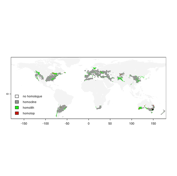
With the homosoil function now established, let’s put it to use. The coordinates below correspond to a location which here is Canberra, Australia .

## SITE LOCATION (Canberra, Australia)
recipient.lat = -35.2809
recipient.lon = 149.13

Now we run the homosoil function.

## RUN FUNCTION
result <- homosoil(grid_data = homosoil_globeDat, recipient.lon = recipient.lon, recipient.lat = recipient.lat)

Then we plot the result. Here we want to use the map object that was created inside the homosoil function. We also specify colors to correspond the non-homologue areas, homoclines, homoliths, and homotops. Because of the hierarchical nature of the homosoil analysis, essentially the homotops are the soil homologues to the recipient site.

# get the map
map.out <- result[[1]]
crs(map.out) <- "+init=epsg:4326"

# plot
levels(map.out) = data.frame(value = 0:3, desc = c("no homologue", "homocline", "homolith", "homotop"))

area_colors <- c("#f4f4f4", "#969895", "#1CEB15", "#C91601")

terra::plot(map.out, col = area_colors, plg = list(legend = c("no homologue", "homocline", "homolith", "homotop"), x = "bottomleft", cex = 0.8))

# plot point
pt1 = sf::st_point(c(recipient.lon, recipient.lat))
plot(pt1, add = T, col = "#040404", pch = 16, cex = 0.8)

rconsole — Soil homologues of soils at Canberra, Australia (black dot on map).

Using the other object that is returned from the homosoil function (which was the world.grid data frame used to put the analysis outputs into) we can also map out the homologues individually, for example, we may just want to map the homoclines. It is always fun just to play around with the function to try out different locations and see what corresponding homologues are found. The results might be surprising. However, the resolution of the data is limiting, so please take this into consideration.

References

Bui, E N, B L Henderson, and K. Viergever. 2006. “Knowledge Discovery from Models of Soil Properties Developed Through Data Mining.” Ecological Modelling 191: 431–46.

Gower, J C. 1971. “A General Coefficient of Similarity and Some of Its Properties.” Biometrics 27: 857–71.

Mallavan, B P, B Minansy, and A B. McBratney. 2010. “Digital Soil Mapping: Bridging Reseach, Environmental Application, and Operation.” In, edited by J L Boettinger, D W Howell, A C Moore, and S. Hartemink A E Kienast-Brown, 137–49. New York: Springer.