CODE:
Get the code used for this section here
Multinomial logistic regression
Introduction
Multinomial logistic regression is used to model nominal outcome variables, in which the log odds of the outcomes are modeled as a linear combination of the predictor variables.
Because we are dealing with categorical variables, it is necessary that logistic regression take the natural logarithm of the odds (log-odds) to create a continuous criterion. The logit of success is then fit to the predictors using regression analysis.
The results of the logit, however are not intuitive, so the logit is converted back to the odds via the inverse of the natural logarithm, namely the exponential function. Therefore, although the observed variables in logistic regression are categorical, the predicted scores are modeled as a continuous variable (the logit). The logit is referred to as the link function in logistic regression.
Although the output in logistic regression will be binomial or multinomial, the logit is an underlying continuous criterion upon which linear regression is conducted. This means that for logistic regression we are able to return the most likely or probable prediction (class) as well as the probabilities of occurrence for all the other classes considered. Some discussion of the theoretical underpinnings of multinomial logistic regression, and importantly its application in DSM is given in Kempen et al. (2009).
Data Preparation
In R we can use the multinom function from the nnet package to perform logistic regression. The are other implementations of this model in R, so it is worth a look to compare and contrast them. Fitting multinom is just like fitting a linear model as seen below.
As described earlier, the data to be used for the following modelling exercises are Terron classes as sampled from the map presented in Malone et al. 2014.The sample data contains 1000 cases of which there are 12 different Terron classes. Before getting into the modeling, we first load in the data and then perform the covariate layer intersection using the suite of environmental variables sourced from the ithir package.
The small selection of covariates cover an area of approximately 220km2 at a spatial resolution of 25m. All these variables are derived primarily from an available digital elevation model.
## load libraries
library(ithir)
library(sf)
library(terra)
library(nnet)

# point data of terron classifications
data(hvTerronDat)

# environmental covariates grids (covariate rasters from ithir package)
hv.rasters <- list.files(path = system.file("extdata/", package = "ithir"), pattern = "hunterCovariates_A", full.names = T)

# read them into R as SpatRaster objects
hv.rasters <- terra::rast(hv.rasters)
Transform the hvTerronDat data to a sf object or simple feature collection which will permit spatial analysis to tak place.
hvTerronDat <- sf::st_as_sf(x = hvTerronDat, coords = c("x", "y"))
As these data are of the same spatial projection as the raster data, there is no need to perform a coordinate transformation. So we can perform the intersection immediately.
## Covariate data extraction
DSM_data <- terra::extract(x = hv.rasters, y = hvTerronDat, bind = T, method = "simple")
DSM_data <- as.data.frame(DSM_data)
str(DSM_data)

## 'data.frame':    1000 obs. of  9 variables:
It is always good practice to check to see if any of the observational data returned any NA values for any one of the covariates. If there is NA values, it indicates that the observational data is outside the extent of the covariate layers. It is best to remove these observations from the data set.
## remove missing data
which(!complete.cases(DSM_data))

## integer(0)

DSM_data <- DSM_data[complete.cases(DSM_data), ]
Model Fitting
Now for model fitting. The target variable is terron. So lets just use all the available covariates in the model. We will also subset the data for an out-of-bag model evaluation using the random hold back sampling method.
# Multinomial logistic regression model establish calibration and out-of-bag
# data sets
set.seed(655)
training <- sample(nrow(DSM_data), 0.7 * nrow(DSM_data))

# Multinomial logistic regression model
hv.MNLR <- nnet::multinom(terron ~ hunterCovariates_A_AACN + hunterCovariates_A_elevation + hunterCovariates_A_Hillshading + hunterCovariates_A_light_insolation + hunterCovariates_A_MRVBF + hunterCovariates_A_Slope + hunterCovariates_A_TRI + hunterCovariates_A_TWI, data = DSM_data[training, ])
Using the summary function allows us to see the linear models for each Terron class, which are the result of the log-odds of each soil class modeled as a linear combination of the covariates. We can also see the probabilities of occurrence for each Terron class at each observation location by using the fitted function.
## Model summary
summary(hv.MNLR)

## Call:
## nnet::multinom(formula = terron ~ hunterCovariates_A_AACN + hunterCovariates_A_elevation +
##     hunterCovariates_A_Hillshading + hunterCovariates_A_light_insolation +
##     hunterCovariates_A_MRVBF + hunterCovariates_A_Slope + hunterCovariates_A_TRI +
##     hunterCovariates_A_TWI, data = DSM_data[training, ])
##
## Coefficients:
#
##
## Residual Deviance: 1565.641
## AIC: 1763.641

# Estimate class probabilities
probs.hv.MNLR <- fitted(hv.MNLR)

# return top of data frame of probabilities
head(probs.hv.MNLR)

##                1            2            3            4            5
## 366 3.180013e-07 6.777814e-03 4.903625e-01 0.0001686759 0.0001705747
## 79  1.494619e-06 8.747864e-07 3.335882e-03 0.0358131506 0.0226158580
## 946 7.747219e-07 1.390212e-05 3.110918e-03 0.0063934663 0.0814475628
## 148 8.990125e-09 6.399129e-10 2.020176e-07 0.0116442200 0.5644019303
## 710 5.758595e-04 3.707932e-03 6.952536e-01 0.0103778544 0.0001168495
## 729 1.232164e-11 8.209651e-10 4.582702e-08 0.0003529924 0.4953536210
##
Subsequently, we can also determine the most probable Terron class using the predict function.
## model prediction
pred.hv.MNLR <- predict(hv.MNLR)
summary(pred.hv.MNLR)

##   1   2   3   4   5   6   7   8   9  10  11  12
##  20   6  82  42 111  61 143 122  47  28  24  14
Model goodness of fit evaluation
Lets now perform an internal validation of the model to assess its general performance. Here we use the goofcat function that was introduced earlier, but this time we import the two vectors into the function which correspond to the observations and predictions respectively.
## goodness of fit (calibration)
ithir::goofcat(observed = DSM_data$terron[training], predicted = pred.hv.MNLR)

## $confusion_matrix
##     1 2  3  4  5  6  7  8  9 10 11 12
## 1  14 0  0  2  0  0  0  0  3  1  0  0
## 2   0 5  1  0  0  0  0  0  0  0  0  0
## 3   0 4 43  2  0  0 12  0  0  0  8 13
## 4   4 0  3 22  2  1  3  1  5  0  1  0
## 5   0 0  0  0 60 17  3  0  7 19  3  2
## 6   0 0  0  0 13 42  0  4  0  2  0  0
## 7   1 0 12  7  2  0 72 18  2 13  3 13
## 8   0 0  0  1  1  6 19 80  0  7  8  0
## 9   0 0  0  8  3  0  5  1 29  0  0  1
## 10  0 0  0  1  9  0  4  1  0 12  1  0
## 11  0 0  9  0  1  1  0  4  0  0  9  0
## 12  0 0  4  0  1  0  4  0  0  0  0  5
##
## $overall_accuracy
## [1] 57
##
## $producers_accuracy
##  1  2  3  4  5  6  7  8  9 10 11 12
## 74 56 60 52 66 63 60 74 64 23 28 15
##
## $users_accuracy
##  1  2  3  4  5  6  7  8  9 10 11 12
## 70 84 53 53 55 69 51 66 62 43 38 36
##
## $kappa
## [1] 0.5023977
Similarly, performing the out-of-bag evaluation requires first using the pred.hv.MNLR model to predict on the out-of-bag cases.
## goodness of fit (out-of-bag)
V.pred.hv.MNLR <- predict(hv.MNLR, newdata = DSM_data[-training, ])

ithir::goofcat(observed = DSM_data$terron[-training], predicted = V.pred.hv.MNLR)

## $confusion_matrix
##    1 2  3  4  5  6  7  8  9 10 11 12
## 1  5 0  0  1  0  0  1  0  1  0  0  0
## 2  1 0  0  0  0  0  0  0  0  0  0  0
## 3  0 4 15  5  0  0  3  0  0  2  2  3
## 4  2 0  1 11  0  1  1  0  0  0  0  0
## 5  0 0  0  3 24  4  0  2  2  2  2  0
## 6  0 0  0  0  7 17  0  2  1  0  0  0
## 7  0 0  6  7  2  0 33  8  3  4  8  3
## 8  0 0  0  1  1  3  6 26  1  5  0  1
## 9  0 0  1  2  1  0  3  0 12  0  0  0
## 10 0 0  0  0  5  0  1  0  0 10  0  3
## 11 0 0  3  2  0  0  0  3  0  0  3  0
## 12 0 0  1  0  0  0  5  0  0  1  0  1
##
## $overall_accuracy
## [1] 53
##
## $producers_accuracy
##  1  2  3  4  5  6  7  8  9 10 11 12
## 63  0 56 35 60 68 63 64 60 42 20 10
##
## $users_accuracy
##  1  2  3  4  5  6  7  8  9 10 11 12
## 63  0 45 69 62 63 45 60 64 53 28 13
##
## $kappa
## [1] 0.4600514
Apply model spatially
Using the terra::predict function is the method for applying the hv.MNLR model across the whole area. Model extension can take a couple of forms for MNLR. It is possible for multinomial logistic regression to create the map of the most probable class, as well as the probabilities for all classes. The first script example below is for mapping the most probable class which is specified by setting the type parameter to
class. If probabilities are required probs would be used for the type parameter, together with specifying an index integer to indicate which class probabilities you wish to map.
The second script example below shows the parametisation for predicting the probabilities for Terron class 1.
## Apply model spatially class prediction
map.MNLR.c <- terra::predict(object = hv.rasters, model = hv.MNLR, type = "class")

# class probabilities (for estimation of Terron 1)
map.MNLR.p <- terra::predict(object = hv.rasters, model = hv.MNLR, type = "probs", index = 1)
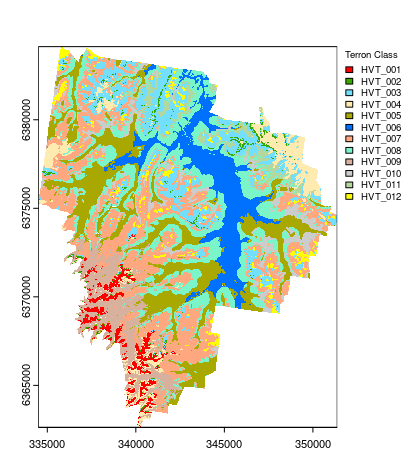
Plotting the final map is done as below. You will also note the use of explicit colors for each Terron class as they were the same colors used in the Terron map presented by Malone et al. (2014). The colors are defined in terms of HEX color codes. A very good resource for selecting colors or deciding on color ramps for maps is colorbrewer.
## Plotting
map.MNLR.c <- as.factor(map.MNLR.c)

## HEX colors
area_colors <- c("#FF0000", "#38A800", "#73DFFF", "#FFEBAF", "#A8A800", "#0070FF", "#FFA77F", "#7AF5CA", "#D7B09E", "#CCCCCC", "#B4D79E", "#FFFF00")

terra::plot(map.MNLR.c, col = area_colors, plg = list(legend = c("HVT_001", "HVT_002", "HVT_003", "HVT_004", "HVT_005", "HVT_006", "HVT_007", "HVT_008", "HVT_009", "HVT_010", "HVT_011", "HVT_012"), cex = 0.75, title = "Terron Class"))
References
Kempen, B, D. J Brus, G. B. M Heuvelink, and J. J Stoorvogel. 2009. “Updating the 1:50,000 Dutch Soil Map Using Legacy Soil Data: A Multinomial Logistic Regression Approach.” Geoderma 151: 311–26.
Malone, B P, P Hughes, A B McBratney, and B Minsany. 2014. “A Model for the Identification of Terrons in the Lower Hunter Valley, Australia.” Geoderma Regional 1: 31–47.