Cubist Models

CODE:

Digital soil mapping using Cubist model algorithm

Introduction
Data preparation
Perform the covariate intersection
Model fitting
Cross-validation
Applying the model spatially

Introduction

The Cubist model is a popular model algorithm used throughout the DSM community. Its popularity is due to its ability to mine non-linear relationships in data, but does not have the issues of finite predictions that occur for other decision and regression tree models. In similar vain to regression trees however, Cubist models also are a data partitioning algorithm. The Cubist model is based on the M5 algorithm of Quinlan (1992), and is implemented in the R Cubist package.

The Cubist model first partitions the data into subsets within which their characteristics are similar with respect to the target variable and the covariates. A series of rules (a decision tree structure may also be defined if requested) defines the partitions, and these rules are arranged in a hierarchy. Each rule takes the form:

if [condition is true]
then [regress]
else [apply the next rule]

The condition may be a simple one based on one covariate or, more often, it comprises several covariates. If a condition results in being true then the next step is the prediction of the soil property of interest by ordinary least-squares regression from the covariates within that partition.

If the condition is not true then the rule defines the next node in the tree, and the sequence of if, then, else is repeated. The result is that the regression equations, though general in form, are local to the partitions and their errors smaller than they would otherwise be. More details of the Cubist model can be found in the Cubist help files or Quinlan (1992).

Fitting a Cubist model in R is not very difficult. Although it will be useful to spend some time playing around with many of the controllable hyper-parameters the function has.

In the example below we can control the number of potential rules that could potentially partition the data (note this limits the number of possible rules, and does not necessarily mean that those number of rules will actually be realized i.e. the outcome is internally optimized). We can also limit the extrapolation of the model predictions, which is a useful model constraint feature. These various control parameters plus others can be adjusted within the cubistControl parameter. The committees parameter is specified as an integer of how many committee models (e.g.. boosting iterations) are required. Here we just set it to 1, but naturally it is possible to perform some sort of sensitivity analysis when this committee model option is set to greater than 1. In terms of specifying the target variable and covariates, we do not define a formula as we did earlier for the MLR model. Rather we specify the columns explicitly — those that are the target variable (x), and those that are the covariates (y).

Data preparation

So lets firstly get the data organized. Recall from before in the data preparatory exercises that we were working with the soil point data and environmental covariates for the Hunter Valley area. These data are stored in the HV_subsoilpH object and supplied rasters from the ithir package.

For the succession of models examined in these various pages, we will concentrate on modelling and mapping the soil pH for the 60-100cm depth interval. To refresh, lets load the data in, then intersect the data with the available covariates.

library(ithir)
library(terra)
library(sf)
library(Cubist)

# point data
data(HV_subsoilpH)

# Start afresh round pH data to 2 decimal places
HV_subsoilpH$pH60_100cm <- round(HV_subsoilpH$pH60_100cm, 2)

# remove already intersected data
HV_subsoilpH <- HV_subsoilpH[, 1:3]

# add an id column
HV_subsoilpH$id <- seq(1, nrow(HV_subsoilpH), by = 1)

# re-arrange order of columns
HV_subsoilpH <- HV_subsoilpH[, c(4, 1, 2, 3)]

# Change names of coordinate columns
names(HV_subsoilpH)[2:3] <- c("x", "y")
# save a copy of coordinates
HV_subsoilpH$x2 <- HV_subsoilpH$x
HV_subsoilpH$y2 <- HV_subsoilpH$y

# convert data to sf object
HV_subsoilpH <- sf::st_as_sf(x = HV_subsoilpH, coords = c("x", "y"))

# grids (covariate rasters from ithir package)
hv.sub.rasters <- list.files(path = system.file("extdata/", package = "ithir"), pattern = "hunterCovariates_sub", full.names = TRUE)

# read them into R as SpatRaster objects
hv.sub.rasters <- terra::rast(hv.sub.rasters)

Perform the covariate intersection

DSM_data <- terra::extract(x = hv.sub.rasters, y = HV_subsoilpH, bind = T, method = "simple")
DSM_data <- as.data.frame(DSM_data)

Often it is handy to check to see whether there are missing values both in the target variable and of the covariates. It is possible that a point location does not fit within the extent of the available covariates. In these cases the data should be excluded. A quick way to assess whether there are missing or NA values in the data is to use the complete.cases function.

# check for NA values
which(!complete.cases(DSM_data))

## integer(0)

DSM_data <- DSM_data[complete.cases(DSM_data), ]

There do not appear to be any missing data as indicated by the integer(0) output above i.e there are zero rows with missing information.

Model Fitting

Before fitting the model, like other previous examples, we first perform a random hold-back sub-sampling to use for an external validation .

## Cubist model fitting 
# select a random set by holdback for model calibration
set.seed(875)
training <- sample(nrow(DSM_data), 0.7 * nrow(DSM_data))
mDat <- DSM_data[training, ]

# fit the model
hv.cub.Exp <- Cubist::cubist(x = mDat[, c("AACN", "Landsat_Band1", "Elevation", "Hillshading",
"Mid_Slope_Positon", "MRVBF", "NDVI", "TWI")], y = mDat$pH60_100cm, cubistControl(rules = 100,
extrapolation = 15), committees = 1)

The output generated from fitting a Cubist model can be retrieved using the summary function. This provides information about the conditions for each rule, the regression models for each rule, and information about the diagnostics of the model fit, plus the frequency of which the covariates were used as conditions and/or within a model.

summary(hv.cub.Exp)

## 
## Call:
## cubist.default(x = mDat[, c("AACN", "Landsat_Band1",
##  = mDat$pH60_100cm, committees = 1, control = cubistControl(rules =
##  100, extrapolation = 15))
## 
## 
## Cubist [Release 2.07 GPL Edition]  Wed Sep 13 10:28:18 2023
## ---------------------------------
## 
##     Target attribute `outcome'
## 
## Read 354 cases (9 attributes) from undefined.data
## 
## Model:
## 
##   Rule 1: [354 cases, mean 6.486, range 3 to 9.74, est err 0.947]
## 
##  outcome = 7.376 + 0.48 MRVBF + 0.0188 AACN + 4.9 NDVI
##            + 0.076 Hillshading - 0.038 Landsat_Band1
##            + 0.96 Mid_Slope_Positon
## 
## 
## Evaluation on training data (354 cases):
## 
##     Average  |error|              1.128
##     Relative |error|               1.03
##     Correlation coefficient        0.33
## 
## 
##  Attribute usage:
##    Conds  Model
## 
##           100%    AACN
##           100%    Landsat_Band1
##           100%    Hillshading
##           100%    Mid_Slope_Positon
##           100%    MRVBF
##           100%    NDVI
## 
## 
## Time: 0.0 secs

The useful feature of the Cubist model is that it does not unnecessarily over fit and partition the data, although you do need to keep an eye on the number of observations within each rule set. Lets evaluate the model.

Cross-validation

## Goodness of fit model evaluation Internal validation
Cubist.pred.C <- predict(hv.cub.Exp, newdata = DSM_data[training, ])
goof(observed = DSM_data$pH60_100cm[training], predicted = Cubist.pred.C)

##          R2 concordance      MSE     RMSE       bias
## 1 0.2451631    0.390694 1.353835 1.163544 -0.1086524

# External validation
Cubist.pred.V <- predict(hv.cub.Exp, newdata = DSM_data[-training, ])
goof(observed = DSM_data$pH60_100cm[-training], predicted = Cubist.pred.V)

##          R2 concordance      MSE     RMSE        bias
## 1 0.1978859     0.33224 1.506298 1.227313 -0.05218972

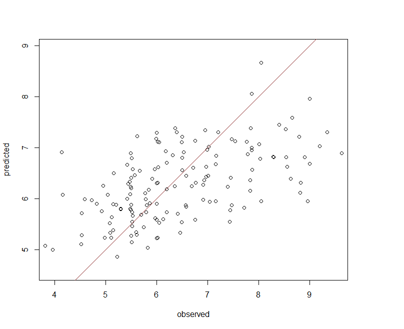
The calibration model validates quite well, but its performance against the validation is comparable. From Figure below it appears a few observations are under predicted (negative bias), otherwise the Cubist model performs reasonably well.

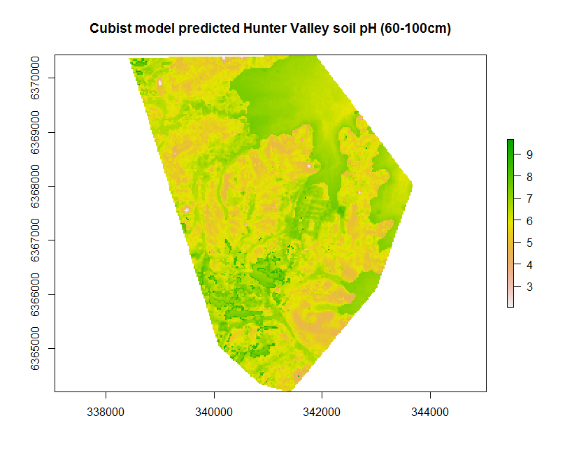
rconsole — Cubist model xy-plot plot of predicted soil pH (60-100cm) (validation data set).

Spatial prediction

Creating the map resulting from the hv.cub.Exp model can be implemented as before using the terra::predict function.

## Spatial prediction
map.cubist.r1 <- terra::predict(object = hv.sub.rasters, model = hv.cub.Exp, filename = "soilpH_60_100_cubist.tif", datatype = "FLT4S", overwrite = TRUE)

plot(map.cubist.r1, main = "Cubist model predicted Hunter Valley soil pH (60-100cm)")

References

Quinlan, J R. 1992. “Proceedings of Ai92, 5th Australian Conference on Artificial Intelligence, Singapore.” In, edited by A Adams and L Sterling, 343–48. World Scientific.