CODE:
Get the code used for this section here
Multiple linear regression model applied to digital soil mapping
- Introduction
- Data preparation
- Perform the covariate intersection
- Model fitting (full model)
- Model fitting (step-wise covariate selection)
- Cross-validation
- Applying the model spatially
- Other possible spatial predictions (prediction intervals)
Introduction
Multiple linear regression (MLR) is where we regress a target variable against more than one covariate. In terms of soil spatial prediction functions, MLR is a least-squares model whereby we want to to predict a continuous soil variable from a suite of covariates.
There are a couple of ways to go about this. We could just put everything (all the covariates) in the model and then fit it (estimate the model parameters).
We could also perform a step-wise regression model where we only enter variables that are statistically significant, based on some selection criteria.
Alternatively we could fit what could be termed, an ‘expert’ model, such that based on some pre-determined knowledge of the soil variable we are trying to model, we include covariates that best describe this knowledge. In some ways this is a biased model because we really don’t know everything about (the spatial characteristics) the soil property under investigation. Yet in many situations it is better to rely on expert knowledge that is gained in the field as opposed to a purely data driven approach.
Data preparation
So lets firstly get the data organized. Recall from before in the data preparatory exercises that we were working with the soil point data and environmental covariates for the Hunter Valley area. These data are stored in the HV_subsoilpH object and supplied raster files from the ithir package.
For the succession of models examined in these various pages, we will concentrate on modelling and mapping the soil pH for the 60-100cm depth interval. To refresh, lets load the data in, then intersect the data with the available covariates.
# load libraries
library(ithir)
library(terra)
library(sf)
library(viridis)

# point data
data(HV_subsoilpH)

# Start afresh round pH data to 2 decimal places
HV_subsoilpH$pH60_100cm <- round(HV_subsoilpH$pH60_100cm, 2)

# remove already intersected data
HV_subsoilpH <- HV_subsoilpH[, 1:3]

# add an id column
HV_subsoilpH$id <- seq(1, nrow(HV_subsoilpH), by = 1)

# re-arrange order of columns
HV_subsoilpH <- HV_subsoilpH[, c(4, 1, 2, 3)]

# Change names of coordinate columns
names(HV_subsoilpH)[2:3] <- c("x", "y")
# save a copy of coordinates
HV_subsoilpH$x2 <- HV_subsoilpH$x
HV_subsoilpH$y2 <- HV_subsoilpH$y

# convert data to sf object
HV_subsoilpH <- sf::st_as_sf(x = HV_subsoilpH, coords = c("x", "y"))

# grids (covariate rasters from ithir package)
hv.sub.rasters <- list.files(path = system.file("extdata/", package = "ithir"), pattern = "hunterCovariates_sub", full.names = TRUE)

# read them into R as SpatRaster objects
hv.sub.rasters <- terra::rast(hv.sub.rasters)
Perform the covariate intersection
DSM_data <- terra::extract(x = hv.sub.rasters, y = HV_subsoilpH, bind = T, method = "simple")
DSM_data <- as.data.frame(DSM_data)
Often it is handy to check to see whether there are missing values both in the target variable and of the covariates. It is possible that a point location does not fit within the extent of the available covariates. In these cases the data should be excluded. A quick way to assess whether there are missing or NA values in the data is to use the complete.cases function.
which(!complete.cases(DSM_data))

## integer(0)

DSM_data <- DSM_data[complete.cases(DSM_data), ]
There do not appear to be any missing data as indicated by the integer(0) output above i.e there are zero rows with missing information.
Model fitting (full model)
With the soil point data prepared, lets fit a model with everything in it (all covariates) to get an idea of how to parameterise the MLR models in R. Remember the soil variable we are making a model for is soil pH for the 60-100cm depth interval.
hv.MLR.Full <- lm(pH60_100cm ~ +Terrain_Ruggedness_Index + AACN + Landsat_Band1 +
Elevation + Hillshading + Light_insolation + Mid_Slope_Positon + MRVBF + NDVI +
TWI + Slope, data = DSM_data)
summary(hv.MLR.Full)

##
## Call:
## lm(formula = pH60_100cm ~ +Terrain_Ruggedness_Index + AACN +
##     Landsat_Band1 + Elevation + Hillshading + Light_insolation +
##     Mid_Slope_Positon + MRVBF + NDVI + TWI + Slope, data = DSM_data)
##
## Residuals:
##     Min      1Q  Median      3Q     Max
## -3.2380 -0.7843 -0.1225  0.7057  3.4641
##
## Coefficients:
##                           Estimate Std. Error t value Pr(>|t|)
## (Intercept)               5.372451   2.147673   2.502 0.012689 *
## Terrain_Ruggedness_Index  0.075084   0.054893   1.368 0.171991
## AACN                      0.034747   0.007241   4.798 2.12e-06 ***
## Landsat_Band1            -0.037712   0.009355  -4.031 6.42e-05 ***
## Elevation                -0.013535   0.005550  -2.439 0.015079 *
## Hillshading               0.152819   0.053655   2.848 0.004580 **
## Light_insolation          0.001329   0.001178   1.127 0.260081
## Mid_Slope_Positon         0.928823   0.268625   3.458 0.000592 ***
## MRVBF                     0.324041   0.084942   3.815 0.000154 ***
## NDVI                      4.982413   0.887322   5.615 3.28e-08 ***
## TWI                       0.085150   0.045976   1.852 0.064615 .
## Slope                    -0.102262   0.062391  -1.639 0.101838
## ---
## Signif. codes:  0 '***' 0.001 '**' 0.01 '*' 0.05 '.' 0.1 ' ' 1
##
## Residual standard error: 1.178 on 494 degrees of freedom
## Multiple R-squared:  0.2501, Adjusted R-squared:  0.2334
## F-statistic: 14.97 on 11 and 494 DF,  p-value: < 2.2e-16
Model fitting (step-wise covariate selection)
From the summary output above, it seems a few of the covariates are significant in describing the spatial variation of the target variable. To derive a parsimonious model we could perform a step-wise regression using the step function. With this function we can also specify what direction we want step wise algorithm to proceed.
hv.MLR.Step <- step(hv.MLR.Full, trace = 0, direction = "both")
summary(hv.MLR.Step)

##
## Call:
## lm(formula = pH60_100cm ~ AACN + Landsat_Band1 + Elevation +
##     Hillshading + Mid_Slope_Positon + MRVBF + NDVI + TWI, data = DSM_data)
##
## Residuals:
##     Min      1Q  Median      3Q     Max
## -3.1202 -0.8055 -0.1286  0.7443  3.4407
##
## Coefficients:
##                    Estimate Std. Error t value Pr(>|t|)
## (Intercept)        7.449369   0.930288   8.008 8.36e-15 ***
## AACN               0.037413   0.006986   5.356 1.31e-07 ***
## Landsat_Band1     -0.037795   0.009134  -4.138 4.12e-05 ***
## Elevation         -0.012042   0.005299  -2.273 0.023481 *
## Hillshading        0.089275   0.018576   4.806 2.04e-06 ***
## Mid_Slope_Positon  0.982066   0.263538   3.726 0.000216 ***
## MRVBF              0.307179   0.083361   3.685 0.000254 ***
## NDVI               5.111642   0.882036   5.795 1.21e-08 ***
## TWI                0.092169   0.045241   2.037 0.042149 *
## ---
## Signif. codes:  0 '***' 0.001 '**' 0.01 '*' 0.05 '.' 0.1 ' ' 1
##
## Residual standard error: 1.179 on 497 degrees of freedom
## Multiple R-squared:  0.245,  Adjusted R-squared:  0.2329
## F-statistic: 20.16 on 8 and 497 DF,  p-value: < 2.2e-16
Comparing the outputs of both the full and step-wise MLR models, there is very little difference in the model diagnostics such as the R2. Both models explain about 25% of variation of the target variable.
The ‘full’ model is more complex as it has more parameters than the ‘step’ model. If we apply Occam’s Razor philosophy, the ‘step’ model is preferable.
Cross-validation
As described earlier in the cross-validation page, it is more acceptable to test the performance of a model based upon an external or out-of-bag model evaluation.
Lets fit a new model using the covariates selected in the step wise regression to a random subset of the available data. We will sample 70% of the available rows for the model calibration data set.
set.seed(123)
training <- sample(nrow(DSM_data), 0.7 * nrow(DSM_data))
hv.MLR.rh <- lm(pH60_100cm ~ AACN + Landsat_Band1 + Elevation + Hillshading + Mid_Slope_Positon +
MRVBF + NDVI + TWI, data = DSM_data[training, ])
# calibration predictions
hv.pred.rhC <- predict(hv.MLR.rh, DSM_data[training, ])

# apply predictions to out-of-bag cases
hv.pred.rhV <- predict(hv.MLR.rh, DSM_data[-training, ])
Now we can evaluate the test statistics of the calibration model using the ithir::goof function.
# calibration
goof(observed = DSM_data$pH60_100cm[training], predicted = hv.pred.rhC)

##          R2 concordance      MSE     RMSE          bias
## 1 0.2380964   0.3835304 1.336101 1.155898 -7.105427e-15

# validation
goof(observed = DSM_data$pH60_100cm[-training], predicted = hv.pred.rhV)

##          R2 concordance      MSE     RMSE       bias
## 1 0.2419371   0.3791514 1.445582 1.202323 0.06681039
In this situation the calibration model does not appear to be over fitting because the evaluations for the out-of-bag cases are similar to those of the calibration data. While this is a good result, the prediction model performs only moderately well by the fact there is a noticeable deviation between observations and corresponding model predictions. Examining other candidate models is a way to try to improve upon these results.
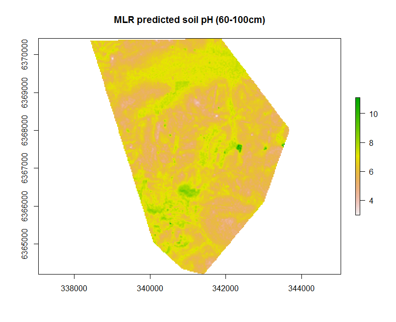
Applying the model spatially
There are a few ways to go about applying a model spatially, but here we will just use the terra::predict function.
In order to eliminate any errors it is necessary to have all the predictive covariates arranged as a stacked SpatRaster object. This is useful as it also ensures all the rasters are of the same extent and resolution. Here we can use the terra::predict function such as below using the hv.sub.rasters loaded earlier.
map.MLR.r1 <- terra::predict(object = hv.sub.rasters, model = hv.MLR.rh, filename = "soilpH_60_100_MLR.tif", datatype = "FLT4S", overwrite = TRUE)
# check working directory for presence of raster
The useful feature of the terra::predict function in this context is that we can write to file directly. This entails leveraging some of the parameters used within the writeRaster function that are worth noting. The parameter datatype is specified as FLT4S which indicates that a 4 byte, signed floating point values are to be written to file. Look at the function dataType to look at other alternatives, for example for categorical data where we may be interested in logical or integer values.
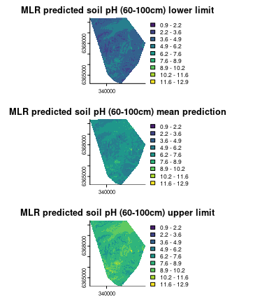
Other possible spatial predictions (prediction intervals)
The prediction function is quite versatile. For example we can also map the standard error of prediction or the confidence interval or the prediction interval even.
The script below is an example of creating maps of the 90% prediction intervals for the model. We need to explicitly create a function called in this case predfun which will direct the terra::predict function to output the predictions plus the upper and lower prediction limits. In the predict function we insert predfun for the fun parameter and control the output by changing the index value to either 1, 2, or 3 to request either the prediction, lower limit, upper limit respectively. Setting the level parameter to 0.90 indicates that we want to return the 90% prediction interval.
# prediction interval function
predfun <- function(model, data) {
v <- terra::predict(model, data, interval = "prediction", level = 0.9)}

# perform the predictions lower prediction limit
map.MLR.r.1ow <- terra::predict(object = hv.sub.rasters, model = hv.MLR.rh, filename = "soilPh_60_100_MLR_low.tif", fun = predfun, index = 2, overwrite = TRUE)

# mean prediction
map.MLR.r.pred <- predict(object = hv.sub.rasters, model = hv.MLR.rh, filename = "soilPh_60_100_MLR_pred.tif", fun = predfun, index = 1, overwrite = TRUE)

# upper prediction limit
map.MLR.r.up <- predict(object = hv.sub.rasters, model = hv.MLR.rh, filename = "soilPh_60_100_MLR_pred.tif", fun = predfun, index = 3, overwrite = TRUE)
# check working directory for presence of rasters

## plot map on the same scale for better comparison stack
stacked.preds <- c(map.MLR.r.1ow, map.MLR.r.pred, map.MLR.r.up)
stacked.preds

rmin <- min(terra::minmax(stacked.preds))
rmax <- max(terra::minmax(stacked.preds))

# plotting parameter
par(mfrow = c(3, 1))

plot(stacked.preds[[1]], col = viridis(10), breaks = seq(rmin, rmax, length.out = 10),
legend = T, bty = "n", box = FALSE, main = "MLR predicted soil pH (60-100cm) lower limit")

plot(stacked.preds[[2]], col = viridis(10), breaks = seq(rmin, rmax, length.out = 10),
legend = T, bty = "n", box = FALSE, main = "MLR predicted soil pH (60-100cm) mean prediction")

plot(stacked.preds[[3]], col = viridis(10), breaks = seq(rmin, rmax, length.out = 10),
legend = T, bty = "n", box = FALSE, main = "MLR predicted soil pH (60-100cm) upper limit")