CODE:
Get the code used in the sections about preparatory and exploratory data analysis
Soil depth functions
Skip to fitting splines to multiple soil profiles
Soil depth functions
The traditional horizon-based sampling method divides a soil profile into discrete layers based on easily observed field properties (e.g., color, texture; Bishop et al. 1999). Each horizon’s bulk sample is assumed to represent the average value of a soil attribute over that depth interval.
However, this approach has two main drawbacks:
- Stepped profiles. Soils vary continuously with depth, but horizon-averaging produces a discontinuous, “stepped” representation.
- Inconsistent depths. Horizon boundaries differ from profile to profile, making it hard to obtain harmonized observations at fixed depths for modelling.
Some one-step models (Orton et al. 2016; Poggio & Gimona 2014) interpolate directly, but most practitioners use a two-step approach:
- Fit a continuous, mass-preserving spline (equal-area quadratic spline) to each profile.
- Extract harmonized values at user-defined depth intervals (e.g. 0–5 cm, 5–15 cm, …, 100–200 cm; GlobalSoilMap.net specification, Arrouays et al. 2014).
A mass-preserving spline has two advantages:
- Data integrity. Total “mass” (integral) over the profile is preserved and recoverable by integration.
- User-defined depths. Spline parameters correspond directly to the soil attribute values at standard depths, enabling easy harmonization across many profiles.
Below, we’ll apply this method to legacy horizon data: fitting splines to each profile and then extracting harmonized values for downstream DSM modelling.
Fit mass preserving splines with R
Skip to fitting splines to multiple soil profiles
The following example shows how to fit a mass-preserving spline to a single soil profile’s carbon-density measurements, from the surface down to its maximum observed depth.
You can choose to fit the spline all the way to the profile’s deepest measurement or to any shallower depth. We use the ea_spline function from the ithir package to perform this fitting.
For details on additional arguments and input types, consult the help file (?ea_spline). Besides data.frame, ea_spline also accepts aqp’s SoilProfileCollection objects when you need more complex profile structures.
In this section, we’ll work with the data.frame called oneProfile (included in ithir). Before running the spline, load ithir and any other supporting packages you’ll need:
#Load ithir library
library(ithir)
#ithir dataset
data(oneProfile)
str(oneProfile)
## 'data.frame': 8 obs. of 4 variables:
## $ Soil.ID : int 1 1 1 1 1 1 1 1
## $ Upper.Boundary: int 0 10 30 50 70 120 250 350
## $ Lower.Boundary: int 10 20 40 60 80 130 260 360
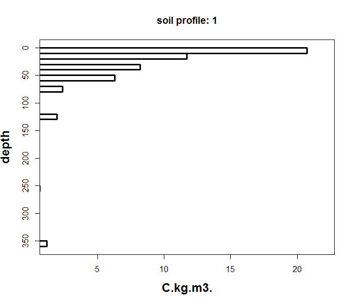
## $ C.kg.m3. : num 20.72 11.71 8.23 6.3 2.4 ...
As you can see above, the data table shows the soil depth information and carbon density values for a single soil profile. Note the discontinuity of the observed depth intervals which can also be observed in the figure below.
The ea_spline function fits a continuous, mass-preserving spline from the soil surface down to your chosen maximum depth. It interpolates smoothly both within observed horizons and across gaps where no measurements exist.
Key parameters
lam(λ): Controls spline smoothness.- Larger values → more rigid (smoother) curves
- Smaller values → more flexible curves that follow observations closely
- Default: 0.1 (a good starting point for most soil attributes)
- Tip: Perform a simple sensitivity analysis to select an optimal λ for your data.
d: Defines the target depth intervals for harmonized outputs.- Specified as a matrix or vector of breakpoints
- Default intervals (GlobalSoilMap.net): 0–5 cm, 5–15 cm, 15–30 cm, 30–60 cm, 60–100 cm, 100–200 cm
- Tip: Customize these to match your project’s depth requirements.
Workflow:
- Fit the spline to your horizon data.
- Integrate the spline over each interval in
dto obtain harmonized, interval-averaged values.
Below is an example script applying these defaults to the oneProfile data:
eaFit <- ithir::ea_spline(oneProfile, var.name="C.kg.m3.",
        d= t(c(0,5,15,30,60,100,200)),lam = 0.1, vlow=0,
        show.progress=FALSE )
str(eaFit)

## List of 4
##  $ harmonised    :'data.frame':  1 obs. of  8 variables:
##   ..$ id        : num 1
##   ..$ 0-5 cm    : num 21.1
##   ..$ 5-15 cm   : num 15.8
##   ..$ 15-30 cm  : num 9.91
##   ..$ 30-60 cm  : num 7.2
##   ..$ 60-100 cm : num 2.75
##   ..$ 100-200 cm: num 1.72
##   ..$ soil depth: num 360
##  $ obs.preds     :'data.frame':  8 obs. of  6 variables:
##   ..$ Soil.ID       : num [1:8] 1 1 1 1 1 1 1 1
##   ..$ Upper.Boundary: num [1:8] 0 10 30 50 70 120 250 350
##   ..$ Lower.Boundary: num [1:8] 10 20 40 60 80 130 260 360
##   ..$ C.kg.m3.      : num [1:8] 20.72 11.71 8.23 6.3 2.4 ...
##   ..$ predicted     : num [1:8] 19.86 12.46 8.27 6.2 2.56 ...
##   ..$ FID           : num [1:8] 1 1 1 1 1 1 1 1
##  $ splineFitError:'data.frame':  1 obs. of  2 variables:
##   ..$ rmse   : num 0.41
##   ..$ rmseiqr: num 0.0561
##  $ var.1cm       : num [1:200, 1] 21.6 21.4 21.2 20.8 20.3 ...
The ea_spline function returns a list with four elements:
-
harmonised(data.frame):
Predicted spline estimates averaged over your specified depth intervals. -
obs.preds(data.frame):
The original horizon measurements combined with spline-predicted values at those exact depths. splineFitError(data.frame):rmse: root-mean-square error between observations and predictionsnrmse: RMSE normalized by the interquartile range (IQR), providing a scale-independent error metric
var.1cm(matrix):
High-resolution predictions at 1 cm increments down to the maximum depth. Rows correspond to depth (cm), columns to individual profiles.
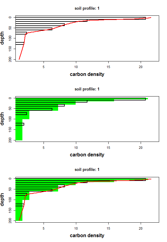
To visualize spline performance, use the accompanying plot_ea_spline function. It offers three plot types:
- Type 1: observed data + continuous spline
- Type 2: observed data + interval means
- Type 3: combined view (continuous spline + interval means)
par(mfrow=c(3,1))
for (i in 1:3){
  ithir::plot_ea_spline(splineOuts=eaFit,
  d= t(c(0,5,15,30,60,100,200)), maxd=200,
  type=i, plot.which=1, label="carbon density")}
The plot_ea_spline function provides three visualization modes, controlled by the type argument:
- Type 1: Observed horizon data with the continuous spline curve (default).
- Type 2: Observed data with interval-averaged spline values at your specified depths.
- Type 3: A combined view showing both the continuous spline and the interval averages.
While plot_ea_spline offers limited customization of axes, labels, or colors, these three themes cover the most common diagnostic needs. The example above loops through all three types, producing a stack of plots like the one shown below.
Fitting spline to multiple soil profiles.
The single-profile example was just a proof of concept. In a typical DSM workflow, you’ll fit splines to many profiles at once. The steps are identical:
- Prepare your data
- Combine all profiles into one
data.frameorSoilProfileCollection. - Include a unique ID column (numeric, character, or mixed) so each profile is processed separately.
- Combine all profiles into one
-
Run the spline fitting
Callea_spline()on your assembled dataset, specifying the object (obj), the target variable (var.name), depth intervals (d), smoothing parameter (lam), minimum value (vlow), and setshow.progress = TRUEto track progress. - Inspect results
eaFit$harmonised: harmonized values per profile & deptheaFit$obs.preds: observed vs. predicted per horizoneaFit$splineFitError: RMSE & nRMSE for each profileeaFit$var.1cm: high-resolution spline curves
For this demo, download Carbon_10sites.csv, which contains 10 profiles of soil carbon measurements.
Performance note: Because
ea_splineuses efficient internal calculations and minimal external dependencies, you can process tens of thousands of profiles in a few minutes. The primary runtime driver is simply the total number of profiles and depth intervals.
# load data
Carbon_10sites<- read.csv("~/Carbon_10sites.csv")

# fit spline to each profile
eaFit <- ithir::ea_spline(obj = Carbon_10sites,
var.name="C.kg.m3.", d= t(c(0,5,15,30,60,100,200)),lam = 0.1, vlow=0, show.progress=FALSE )

str(eaFit)

## List of 4
##  $ harmonised    :'data.frame':  10 obs. of  8 variables:
##   ..$ id        : num [1:10] 1 2 3 4 5 6 7 8 9 10
##   ..$ 0-5 cm    : num [1:10] 28.78 23.68 12.45 7.69 7.51 ...
##   ..$ 5-15 cm   : num [1:10] 18.62 14.67 9.3 6.35 6.94 ...
##   ..$ 15-30 cm  : num [1:10] 10.47 6.48 6.6 5.49 6.47 ...
##   ..$ 30-60 cm  : num [1:10] 9.22 6.65 5.59 5.58 6 ...
##   ..$ 60-100 cm : num [1:10] 5.31 6.13 3.99 4.08 4.41 ...
##   ..$ 100-200 cm: num [1:10] 3.13 3.31 1.18 1.85 2.72 ...
##   ..$ soil depth: num [1:10] 260 260 260 260 260 259 260 260 253 260
##  $ obs.preds     :'data.frame':  62 obs. of  6 variables:
##   ..$ Level.Soil.ID : num [1:62] 1 1 1 1 1 1 2 2 2 2 ...
##   ..$ Upper.Boundary: num [1:62] 0 10 30 70 120 250 0 10 30 70 ...
##   ..$ Lower.Boundary: num [1:62] 8 20 40 80 130 260 10 20 40 80 ...
##   ..$ C.kg.m3.      : num [1:62] 28.69 11.94 10.59 5.28 3.76 ...
##   ..$ predicted     : num [1:62] 27.6 13.06 10.48 5.35 3.77 ...
##   ..$ FID           : num [1:62] 1 1 1 1 1 1 2 2 2 2 ...
##  $ splineFitError:'data.frame':  10 obs. of  2 variables:
##   ..$ rmse   : num [1:10] 0.642 0.6536 0.1653 0.1098 0.0462 ...
##   ..$ rmseiqr: num [1:10] 0.0861 0.2069 0.0321 0.0343 0.0149 ...
##  $ var.1cm       : num [1:200, 1:10] 29.9 29.6 29 28.2 27.2 ...
With multiple profiles, the output becomes more intuitive. In particular, the eaFit$harmonised data frame lists one row per profile, with each column representing the predicted value at a user-specified depth. The soil.depth column gives each profile’s maximum depth, helping you verify that the harmonized estimates cover the full observed range.
References
Arrouays, D., McKenzie, N., Hempel, J., Richer de Forges, A., & McBratney, A. (2014). GlobalSoilMap: Basis of the Global Spatial Soil Information System. CRC Press.
Bishop, T. F. A., McBratney, A. B., & Laslett, G. M. (1999). Modelling soil attribute depth functions with equal-area quadratic smoothing splines. Geoderma, 91, 27–45.
Malone, B. P., McBratney, A. B., Minasny, B., & Laslett, G. M. (2009). Mapping continuous depth functions of soil carbon storage and available water capacity. Geoderma, 154, 138–152.
Orton, T. G., Pringle, M. J., & Bishop, T. F. A. (2016). A one-step approach for modelling and mapping soil properties based on profile data sampled over varying depth intervals. Geoderma, 262, 174–186.
Poggio, L., & Gimona, A. (2014). National-scale 3D modelling of soil organic carbon stocks with uncertainty propagation: an example from Scotland. Geoderma, 232–234, 284–299.
Ponce-Hernandez, R., Marriott, F. H. C., & Beckett, P. H. T. (1986). An improved method for reconstructing a soil profile from analysis of a small number of samples. Journal of Soil Science, 37, 455–467.