CODE:
Get the code used for this section here
R Literacy for digital soil mapping (Part 1 of 8)
Objective
The goal of this first module is to build your skills in data analysis and basic graphics using R. The scope of analysis and visualization possible in R is vast. In addition to the extensive functionality built into the base packages, more than 22,000 contributed packages [as of May 2025] are available on CRAN, with some packages forming the basis of entire books.
This course is split into eight connected parts, starting here. It blends foundational skills—useful even for complete beginners—with specific techniques tailored for digital soil mapping and similar tasks.
This introduction draws inspiration from many freely available online resources. If you get stuck, a quick web search will often turn up helpful advice—chances are, someone else has encountered the same issue.
Given its flexibility, R is not something to “master” like a stand-alone tool, but rather a language in which fluency builds over time. In that sense, learning R is a continuous journey.
Introduction to R
R overview and history
R is a software system for computations and graphics. According to the
R FAQ:
It consists of a language plus a run-time environment with graphics, a debugger, access to certain system functions, and the ability to run programs stored in script files.
R was originally developed in 1992 by Ross Ihaka and Robert Gentleman
at the University of Auckland (New Zealand). The R language is a
dialect of the S language which was developed by John Chambers at Bell
Laboratories. This software is currently maintained by the R
Development Core Team, which consists of more than a dozen people, and
includes Ihaka, Gentleman, and Chambers. Additionally, many other people
have contributed code to R since it was first released. The source
code for R is available under the GNU General Public Licence, meaning
that users can modify, copy, and redistribute the software or
derivatives, as long as the modified source code is made available. R
is regularly updated, however, changes are usually not major.
Finding and installing R
R is available for Windows, Mac, and Linux operating systems.
Installation files and instructions can be downloaded from the
Comprehensive R Archive Network (CRAN). Although the graphical user interface
(GUI) differs slightly across systems, the R commands do not.
Running R: GUI and scripts
There are two basic ways to use R on your machine: through the GUI,
where R evaluates your code and returns results as you work, or by
writing, saving, and then running R script files. R script files (or
scripts) are just text files that contain the same types of R commands
that you can submit to the GUI. Scripts can be submitted to R using
the Windows command prompt, other shells, batch files, or the R GUI.
All the code covered in this workshop is or is able to be saved in a
script file, which then can be submitted to R. Working directly in the
R GUI is great for the early stages of code development, where much
experimentation and trial-and-error occurs. For any code that you want
to save, rerun, and modify, you should consider working with R
scripts.
So, how do you work with scripts? Any simple text editor works—you just
need to save text in the ASCII format i.e. ‘unformatted’ text. You can
save your scripts and either call them up using the command
source ('file_name.R') in the R GUI, or, if you are using a shell
(e.g. Windows command prompt) then type R CMD BATCH file_name.R. The
Windows and Mac versions of the R GUI comes with a basic script
editor, shown below.

Unfortunately, this editor is not very good by reason that the Windows version does not have syntax highlighting.
There are some useful (in most cases, free) text editors available that
can be set up with R syntax highlighting and other features. TINN-R is a
free text editor that is designed
specifically for working with R script files. Notepad++ is a general
purpose text editor, but includes syntax highlighting and the ability to
send code directly to R with the NppToR plugin. A list of text editors
that work well with R can be found at
http://wiki.cbr.washington.edu/qerm/index.php/R/Editors.
RStudio
RStudio is an integrated development environment
(IDE) for R that runs on Linux, Windows and Mac OS X. We will be using
this IDE throughout all the exercises here, generally because it is very
well designed, intuitively organized, and quite stable.
When you first launch RStudio, you will be greeted by an interface that will look similar to that in the figure below.
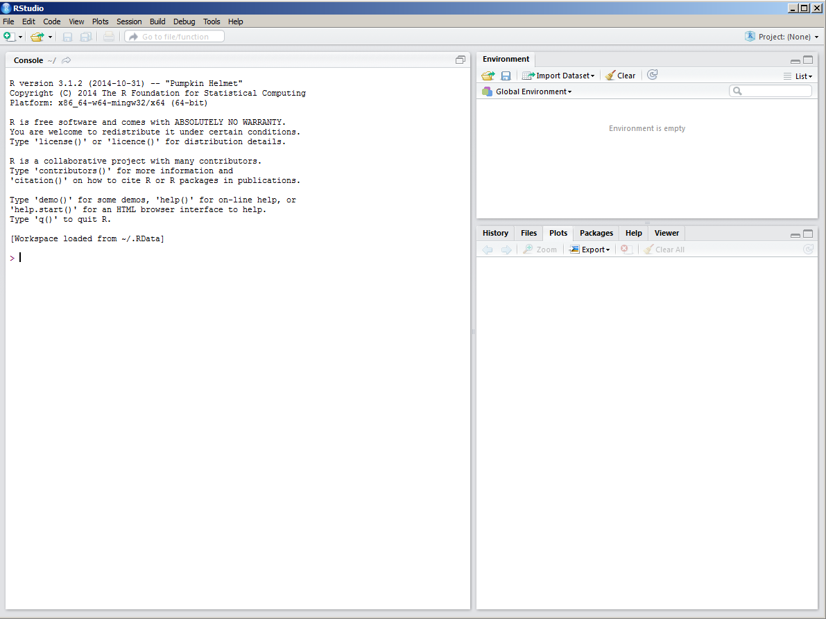
The frame on the upper right contains the workspace (where you will be
able see all your R objects), as well of a history of the commands
that you have previously entered. Any plots that you generate will show
up in the region in the lower right corner. Also in this region is
various help documentation, plus information and documentation regarding
what packages and function are currently available to use .
The frame on the left is where the action happens. This is the R
console. Every time you launch RStudio, it will have the same text at
the top of the console telling you the version that is being used. Below
that information is the prompt. As the name suggests, this is where you
enter commands into R. So lets enter some commands.
R basics: commands, expressions, assignments, operators, objects
Before we start anything, it is good to get into the habit of making
scripts of our work. With RStudio launched go t0 the File menu, then
new, and R Script. A new blank window will open on the top left
panel. Here you can enter your R prompts. For example, type the
following: 1+1. Now roll your pointer over the top of the panel to the
right pointing green arrow (first one), which is a button for running
the line of code down to the R console. Click this button and R will
evaluate it. In the console you should see something like the following:
1+1

## [1] 2
You could have just entered the command directly into the prompt and
gotten the same result. Try it now for yourself. You will notice a
couple of things about this code. The > character is the prompt that
will always be present in the GUI. The line following the command starts
with a [1], which is simply the position of the adjacent element in
the output—this will make some sense later.
For the above command, the result is printed to the screen and
lost—there is no assignment involved. In order to do anything other than
the simplest analyses, you must be able to store and recall data. In
R, you can assign the results of commands to symbolic variables (as in
other computer languages) using the assignment operator <-. Note that
other computer scripting languages often use the equals sign (=) as
the assignment operator. When a command is used for assignment, the
result is no longer printed to the GUI console.
x<- 1+1
x

## [1] 2
Note that this is very different from:
x< -1+1

## [1] FALSE
In this case, putting a space between the two characters that make up
the assignment operator causes R to interpret the command as an
expression that ask if x is less than zero. However spaces usually do
not matter in R, as long as they do not separate a single operator or
a variable name. This, for example, is fine:
x<-   1  +  1
x

## [1] 2
Note that you can recall a previous command in the R GUI by hitting
the up arrow on your keyboard. This becomes handy when you are debugging
code.
When you give R an assignment, such as the one above, the object
referred to as x is stored into the R workspace. You can see what is
stored in the workspace by looking to the workspace panel in RStudio
(top right panel). Alternatively, you can use the ls() function.
ls()

## [1] "x"
To remove objects from your workspace, use rm.
rm(x)
x
As you can see, You will get an error if you try to evaluate what x
is.
If you want to assign the same value to several symbolic variables, you can use the following syntax.
x<-y<-z<- 1.0
ls()

## [1] "x" "y" "z"
R is a case-sensitive language. This is true for symbolic variable
names, function names, and everything else in R.
x<- 1+1
x
X
In R, commands can be separated by moving onto a new line
(i.e. hitting enter) or by typing a semicolon (;), which can be handy in
scripts for condensing code. If a command is not completed in one line
(by design or error), the typical R prompt > is replaced with a +.
x<-
+  1+1
There are several operators that are used in the R language. Some of
the more common are listed below. Until one starts using these
frequently and within context these operators will seem quite foreign.
Arithmetic
+,-,*,/,^equate to plus, minus, multiply, divide, and power operations respectively.
Relational or logical operator
a == bmeans isaequal tob(do not confuse with =).a != bmeans isanot equal tob.a < bmeans isaless thanb.a > bmeans isagreater thanb.a <= bmeans isaless than or equal toba >= bmeans isagreater than or equal tob
Logical/grouping
!not&and|or
Indexing
$index a column of a data frame[]part of a data frame, array, list[[]]part of a list
Grouping commands}
{}specifying a function, for loop, if statement etc.
Making sequences
a:breturns the sequencea,a+1,a+2,...b
Others
#commenting (very very useful!;alternative for separating commands~model formula specification()order of operations, function arguments.
Commands in R operate on objects, which can be thought of as anything that can be assigned to a symbolic variable. Objects include vectors, matrices, factors, lists, data frames, and functions. Excluding functions, these objects are also referred to as data structures or data objects.
When you want to finish up on an R session, RSudio will ask you if you
want to ``save workspace image’’. This refers to the workspace that
you have created , i.e. all the objects you have created or even loaded.
It is generally good practice to save your workspace after each session.
More importantly however, is the need to save all the commands that you
have created on your script file. Saving a script file in Rstudio is
just like saving a Word document. Give both a go—save the script file
and then save the workspace. You can then close RStudio.
R data types
The term ‘data type’ refers to the type of data that is present in a
data structure, and does not describe the data structure itself. There
are four common types of data in R: numerical, character, logical, and
complex numbers. These are referred to as modes and are shown below:
Numerical data
x<- 10.2
x

## [1] 10.2
Character data
name<- "James Carnation"
name

## [1] "James Carnation"
Any time character data are entered in the R GUI, you must surround
individual elements with quotes. Otherwise, R will look for an object.
name<- John
Either single or double quotes can be used in R. When character data
are read into R from a file, the quotes are not necessary.
Logical data
Logical data contain only three values: TRUE, FALSE, or NA, (NA
indicates a missing value - more on this later). R will also recognize
T and F, (for true and false respectively), but these are not
reserved, and can therefore be overwritten by the user, and it is
therefore good to avoid using these shortened terms.
a<- TRUE
a

## [1] TRUE
Note that there are no quotes around the logical values (this would make
them character data). R will return logical data for any relational
expression submitted to it.
4 < 2

## [1] FALSE
or
b<- 4 < 2
b

## [1] FALSE
And finally, complex numbers, which will not be covered in this
workshop, are the final data type in R
cnum1<- 10 + 3i
cnum1

## [1] 10+3i
You can use the mode or class function to see what type of data is
stored in any symbolic variable.
class(name)

## [1] "character"

class(a)

## [1] "logical"

class(x)

## [1] "numeric"

mode(x)

## [1] "numeric"
R data structures
Data in R are stored in data structures (also known as data objects).
These are and will be the things that you perform calculations on, plot
data from, etc. Data structures in R include vectors, matrices,
arrays, data frames, lists, and factors. In a following section we will
learn how to make use of these different data structures. The examples
below simply give you an idea of their structure.
Vectors are perhaps the most important type of data structure in R. A
vector is simply an ordered collection of elements (e.g. individual
numbers).
x<- 1:12
x

##  [1]  1  2  3  4  5  6  7  8  9 10 11 12
Matrices are similar to vectors, but have two dimensions.
X<- matrix(1:12, nrow=3)
X

##      [,1] [,2] [,3] [,4]
## [1,]    1    4    7   10
## [2,]    2    5    8   11
## [3,]    3    6    9   12
Arrays are similar to matrices, but can have more than two dimensions.
Y<- array(1:30,dim=c(2,5,3))
Y

    ## , , 1
    ##
    ##      [,1] [,2] [,3] [,4] [,5]
    ## [1,]    1    3    5    7    9
    ## [2,]    2    4    6    8   10
    ##
    ## , , 2
    ##
    ##      [,1] [,2] [,3] [,4] [,5]
    ## [1,]   11   13   15   17   19
    ## [2,]   12   14   16   18   20
    ##
    ## , , 3
    ##
    ##      [,1] [,2] [,3] [,4] [,5]
    ## [1,]   21   23   25   27   29
    ## [2,]   22   24   26   28   30
One feature that is shared for vectors, matrices, and arrays is that they can only store one type of data at once, be it numerical, character, or logical. Technically speaking, these data structures can only contain elements of the same mode.
Data frames are similar to matrices in that they are two-dimensional. However, a data frame can contain columns with different modes. Data frames are similar to data sets used in other statistical programs: each column represents some variable, and each row usually represents an observation, record, case or experimental unit.
dat<- (data.frame(profile_id= c("Chromosol","Vertosol","Sodosol"),
      FID=c("a1","a10","a11"), easting=c(337859, 344059,347034),
      northing=c(6372415,6376715,6372740), visited=c(TRUE, FALSE, TRUE)))
dat

    ##   profile_id FID easting northing visited
    ## 1  Chromosol  a1  337859  6372415    TRUE
    ## 2   Vertosol a10  344059  6376715   FALSE
    ## 3    Sodosol a11  347034  6372740    TRUE
Lists are similar to vectors, in that they are an ordered collection of elements, but with lists, the elements can be other data objects (the elements can even be other lists). Lists are important in the output from many different functions. In the code below, the variables defined above are used to form a list.
summary.1<- list(1.2, x,Y,dat)
summary.1

    ## [[1]]
    ## [1] 1.2
    ##
    ## [[2]]
    ##  [1]  1  2  3  4  5  6  7  8  9 10 11 12
    ##
    ## [[3]]
    ## , , 1
    ##
    ##      [,1] [,2] [,3] [,4] [,5]
    ## [1,]    1    3    5    7    9
    ## [2,]    2    4    6    8   10
    ##
    ## , , 2
    ##
    ##      [,1] [,2] [,3] [,4] [,5]
    ## [1,]   11   13   15   17   19
    ## [2,]   12   14   16   18   20
    ##
    ## , , 3
    ##
    ##      [,1] [,2] [,3] [,4] [,5]
    ## [1,]   21   23   25   27   29
    ## [2,]   22   24   26   28   30
    ##
    ##
    ## [[4]]
    ##   profile_id FID easting northing visited
    ## 1  Chromosol  a1  337859  6372415    TRUE
    ## 2   Vertosol a10  344059  6376715   FALSE
    ## 3    Sodosol a11  347034  6372740    TRUE
Note that a particular data structure need not contain data to exist. This may seem unusual, but it can be useful when it is necessary to set up an object for holding some data later on.
x<- NULL
# or
x<- c()
Missing, indefinite, and infinite values
Real data sets often contain missing values. R uses the marker NA
(for not available) to indicate a missing value. Any operation carried
out on an NA will return NA.
x<- NA
x-2

## [1] NA
Note that the NA used in R does not have the quotes around it as
this would make it character data. To determine if a value is missing,
use the is.na function.
is.na(x)

## [1] TRUE

!is.na(x)

## [1] FALSE
Indefinite values are indicated with the marker NaN, for not a
number. Infinite values are indicated with the markers Inf or -Inf.
You can find these values with the functions is.infinite, is.finite,
and is.nan.
Functions, arguments, and packages
In R, you can carry out complicated and tedious procedures using
functions. Functions require arguments, which include the object(s) that
the function should act upon. For example, the function sum will
calculate the sum of all of its arguments.
sum(1,12.5,3.33,5,88)

## [1] 109.83
The arguments in (most) R functions can be named, i.e. by typing the
name of the argument, an equal sign, and the argument value (arguments
specified in this way are also called tagged). For example, for the
function plot, the help file lists the following arguments:
plot (x, y,...).
Therefore, we can call up this function with the following code.
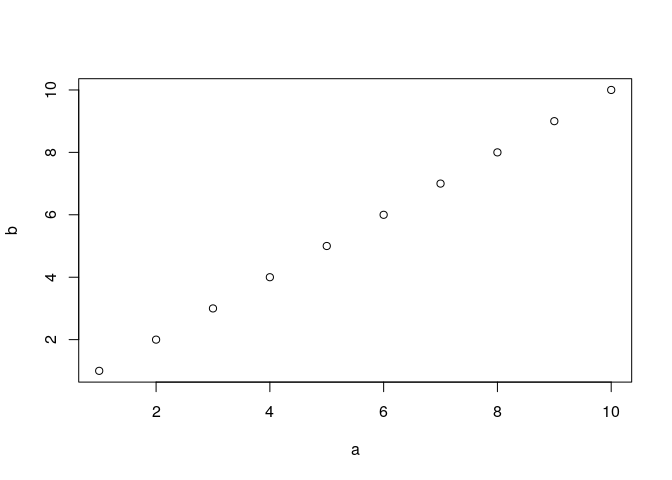
a<- 1:10
b<- a
plot(x=a, y=b)
With named arguments, R recognizes the argument keyword (e.g. x or
y) and assigns the given object (e.g. a or b above) to the correct
argument. When using named arguments, the order of the arguments does
not matter. We can also use what are called positional arguments, where
R determines the meaning of the arguments based on their position.
plot(a, b)
This code does the same as the previous code. The expected position of
arguments can be found in the help file for the function you are working
with or by asking R to list the arguments using the function.
args(plot)

## function (x, y, ...)
## NULL
It usually makes sense to use the positional arguments for only the
first few arguments in a function. After that, named arguments are
easier to keep track of. Many functions also have default argument
values that will be used if values are not specified in the function
call. These default argument values can be seen by using the args
function and can also be found in the help files. For example, for the
function rnorm, the arguments mean and sd have default values.
args(rnorm)

## function (n, mean = 0, sd = 1)
## NULL
Any time you want to call up a function, you must include parentheses
after it, even if you are not specifying any arguments. If you do not
include parentheses, R will return the function code (which at times
might actually be useful).
Note that it is not necessary to use explicit numerical values as
function arguments—symbolic variable names which represent appropriate
data structure can be used. it is also possible to use functions as
arguments within functions. R will evaluate such expressions from the
inside outward. While this may seem trivial, this quality makes R very
flexible. There is no explicit limit to the degree of nesting that can
be used. You could use:
plot(rnorm(10,sqrt(mean(c(1:5, 7,1,8,sum(8.4,1.2,7))))),1:10)
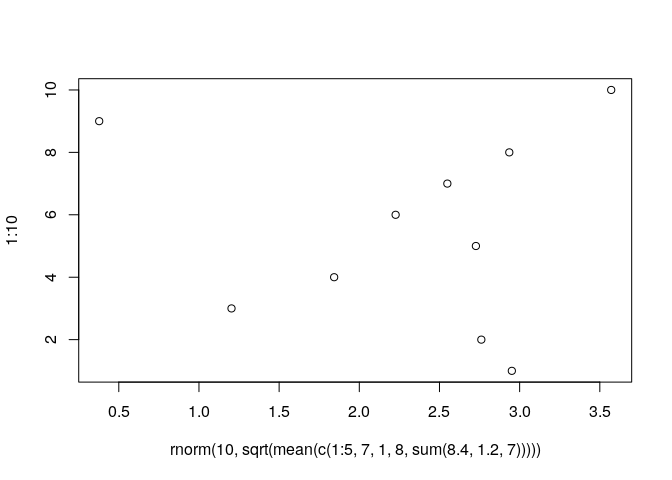
The above code includes 5 levels of nesting (the sum of 8.4,1.2 and 7 is
combined with the other values to form a vector, for which the mean is
calculated, then the square root of this value is taken and used as the
standard deviation in a call to rnorm, and the output of this call is
plotted). Of course, it is often easier to assign intermediate steps to
symbolic variables. R evaluates nested expressions based on the values
that functions return or the data represented by symbolic variables. For
example, if a function expects character data for a particular argument,
then you can use a call to the function paste in place of explicit
character data.
Many functions (including sum, plot, and rnorm) come with the R
base packages, i.e. they are loaded and ready to go as soon as you open
R. These packages contain the most common functions. While the base
packages include many useful functions, for specialized procedures, you
should check out the content that is available in the add-on packages.
The CRAN website currently lists more than 15000 (April 2020)
contributed packages that contain functions and data that users have
contributed. You can find a list of the available packages at the CRAN
website. During the course of these
exercises and described in more detail later on, we will be looking at
and using a number of specialized packages for application of DSM.
Another repository of R packages is the R-Forge
website. R-Forge offers a central
platform for the development of R packages, R-related software and
further projects. Packages in R-Forge are not necessarily always on the
CRAN website. However, many packages on the CRAN website are developed
in R-Forge as ongoing projects. Sometimes to get the latest changes made
upon a package, it pays to visit R-Forge first, as the uploading of the
revised functions to CRAN is not instantaneous. Code repository
platforms such as Github,
Gitlab and
Bitbucket are also important platforms
for developing, maintaining and sharing R packages amongst other
features.
To utilize the functions in contributed R packages, you first need to install and then load the package. Packages can be installed via the packages menu in the right bottom panel of RStudio (select the packages menu, then install packages). Installation could be retrieved from the nearest mirror site (CRAN server location) where you will need to have first selected this by going to the tools, then options, then packages menu where you can then select the nearest mirror site from a suite of possibles. Alternatively, you may just install a package from a local zip file. This is fine, but often when using a package, there are other peripheral packages (or dependencies) that also need to be loaded (and installed). If you install the package from CRAN or a mirror site, the dependency packages are also installed. This is not the case when you are installing packages from zip files—you will also have to manually install all the dependencies too.
Or just use the command:
install.packages("package name")
where package name should be replaced with the actual name of the package you want to install, for example:
install.packages("Cubist")
This command will install the package of functions for running the Cubist rule-based machine learning models for regression which we will come to in later sections
Installation is a one-time process, but packages must be loaded each
time you want to use them. This is very simple, e.g., to load the
package Cubist, use the following command.
library(Cubist)
Similarly, if you want to install an R package from R-Forge (another
popular hosting repository for R packages) you would use the following
command:
install.packages("package name", repos = "http://R-Forge.R-project.org")
Other popular repositories for R packages include
Github and BitBucket.
These repositories as well as R-Forge are version control systems that
provide a central place for people to collaborate on everything from
small to very large projects with speed and efficiency. The companion
R package to these exercises, ithir is hosted on Github for
example. ithir contains most of the data, and some important functions
that are covered in this book so that users can replicate all of the
analyses contained within. ithir can be downloaded and installed on
your computer using the following commands:
library(devtools)
install_bitbucket("brendo1001/ithir_github/pkg")
library(ithir)
The above commands assumes your have already installed the devtools
package. Any package that you want to use that is not included as one of
the “base” packages, needs to be loaded every time you start R.
Alternatively, you can add code to the file Rprofile.site that will be
executed every time you start R.
You can find information on specific packages through CRAN, by browsing
to http://cran.r-project.org/ and selecting the packages link. Each
package has a separate web page, which will include links to source
code, and a pdf manual. In RStudio, you can select the packages tab on
the lower right panel. You will then see all the package that are
currently installed in your R environment. By clicking onto any
package, information on the various functions contained in the package,
plus documentation and manuals for their usage. It becomes quite clear
that within this RStudio environment, there is at your fingertips, a
wealth of information for which to consult whenever you get stuck. When
working with a new package, it is a good idea to read the manual.
To ‘unload’ functions, use the detach function:
detach("package:Cubist")
For tasks that you repeat, but which have no associated function in R,
or if you do not like the functions that are available, you can write
your own functions. This will be covered a little a bit later on.
Perhaps one day you may be able to compile all your functions that you
have created into a R package for everyone else to use.
Getting help
It is usually easy to find the answer about specific functions or about
R in general. There are several good introductory books on R. For
example, R for
Dummies,
which has had many positive reviews. You can also find free detailed
manuals on the CRAN website. Also, it helps to keep a copy of the R
Reference
Card, which
demonstrates the use of many common functions and operators in 4 pages.
Often a Google search of your problem can
be a very helpful and fruitful exercise. To limit the results to R
related pages, adding cran to yoursearch generally works well. R
even has an internet search engine of sorts called
rseek which is really just like the Google search
engine, but just for R stuff!
Each function in R has a help file associated with it that explains
the syntax and usually includes an example. Help files are concisely
written. You can bring up a help file by typing ? and then the
function name.
?cubist
This will bring up the help file for the Cubist function in the help
panel of RStudio. But, what if you are not sure what function you need
for a particular task? How can you know what help file to open? In
addition to the sources given below, you should try
help.search('keyword') or ??keyword, both of which search the R
help files for whatever keyword you put in.
??polygon
This will bring up a search results page in the help panel of RStudio of
all the various help files that have something to do with polygon. In
this case, i am only interested in a function that assesses whether a
point is situated with a polygon. So looking down the list, one can see
(provided the SDMTools package is installed) a function called
pnt.in.poly. Clicking on this function, or submitting ?pnt.in.poly
to R will bring up the necessary help file.
There is an R help mailing list http://www.r-project.org/mail.html,
which can be very helpful. Before posting a question, be sure to search
the mailing list archives, and check the posting guide
http://www.r-project.org/posting-guide.html.
One of the best sources of help on R functions is the mailing list
archives http://cran.r-project.org/, then select search, then
searchable mail archives). Here you can find suggestions for functions
for particular problems, help on using specific functions, and all kinds
of other information. A quick way to search the mailing list archives is
by entering:
RSiteSearch("A Keyword")
For one more trick, to search for objects (including functions) that
include a particular string, you can use the apropos function:
apropos("mean")
Exercises
-
You can use for magic tricks: Pick any number. Double it, and then add 12 to the result. Divide by 2, and then subtract your original number. Did you end up with 6.0?
-
If you want to work with a set of 10 numbers in
R, something like this:11, 8.3, 9.8, 9.6, 11.0, 12.0, 8.5, 9.9, 10.0,11.0
- What type of data structure should you use to store these in
R? - What if you want to work with a data set that contains site names,
site locations, soil categorical information, soil property
information, and some terrain variables—what type of data structure
should you use to store these in
R?
-
Install and load a package—take a look at the list of available packages, and pick one. To make sure you have loaded it correctly, try to run an example from the package reference manual. Identify the arguments required for calling up the function. Detach the package when you are done.
-
Assign your full name to a variable called
my.name. Print the value ofmy.name. Try to subtract 10 frommy.name. Finally determine the type of data stored inmy.nameand 10 using theclassfunction. If you are unsure of whatclassdoes, check out the help file. -
You are interested in seeing what functions
Rhas for fitting variograms (or some other topic of your choosing). Can you figure out how to search for relevant functions? Are you able to identify a function or two that may do what you want.