CODE:
Get the code used for this section here
Exploratory data analysis
Summary statistics
We will again use the soil.data set to demonstrate calculation of
summary statistics. Just for recall, lets see what is in this data
frame.
    library(ithir)
    data(USYD_soil1)
    soil.data <- USYD_soil1
    names(soil.data)

    ##  [1] "PROFILE"      "Landclass"    "Upper.Depth"  "Lower.Depth"  "clay"
    ##  [6] "silt"         "sand"         "pH_CaCl2"     "Total_Carbon" "EC"
    ## [11] "ESP"          "ExchNa"       "ExchK"        "ExchCa"       "ExchMg"
    ## [16] "CEC"
Here are some useful functions (and note the usage of the na.rm
argument) for calculation of means (mean), medians (median),
standard deviations (sd) and variances (var):
    mean(soil.data$clay, na.rm = TRUE)

    ## [1] 26.95302

    median(soil.data$clay, na.rm = TRUE)

    ## [1] 21

    sd(soil.data$clay, na.rm = TRUE)

    ## [1] 15.6996

    var(soil.data$clay, na.rm = TRUE)

    ## [1] 246.4775
R has a built-in function for summarizing vectors or data frames
called summary. This function is a generic function—what it returns is
dependent on the type of data set to it. Applying the summary function
to the first 6 columns in the soil.data set results in the following
output:
    summary(soil.data[, 1:6])

    ##     PROFILE                 Landclass   Upper.Depth      Lower.Depth
    ##  Min.   : 1.00   Cropping        :49   Min.   :0.0000   Min.   :0.0200
    ##  1st Qu.: 8.00   Forest          :50   1st Qu.:0.0200   1st Qu.:0.0500
    ##  Median :15.00   improved pasture:35   Median :0.0500   Median :0.1000
    ##  Mean   :14.73   native pasture  :32   Mean   :0.1816   Mean   :0.2464
    ##  3rd Qu.:22.00                         3rd Qu.:0.2000   3rd Qu.:0.3000
    ##  Max.   :29.00                         Max.   :0.7000   Max.   :0.8000
    ##
    ##       clay            silt
    ##  Min.   : 5.00   Min.   : 6.0
    ##  1st Qu.:15.00   1st Qu.:11.0
    ##  Median :21.00   Median :15.0
    ##  Mean   :26.95   Mean   :16.5
    ##  3rd Qu.:37.00   3rd Qu.:20.0
    ##  Max.   :68.00   Max.   :32.0
    ##  NA's   :17      NA's   :1
Notice the difference between numerical and categorical variables. The
summary function should probably be your first stop after organizing
your data, and before analyzing it as it provides an easy way to check
for wildly erroneous values.
Histograms and box plots
Box plots and histograms are simple but useful ways of summarizing data.
You can generate a histogram in R using the function hist.
hist(soil.data$clay)
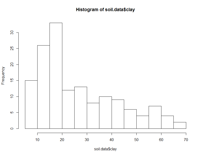
The histogram above can be made to look nicer, by applying some of the
plotting parameters or arguments that were covered in Part 4 about the
plot function. There are also some additional plotting arguments
that can be sourced in the hist help file. One of these is the ability
to specify the number or location of breaks in the histogram.
Box plots are also a useful way to summarize data. We can use it simply,
for example, summarize the clay content in the soil.data:
boxplot(soil.data$clay)
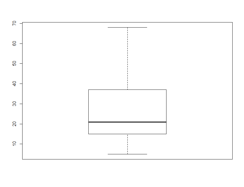
By default, the heavy line shows the median, the box shows the 25t**h and 75t**h percentiles, the whiskers show the extreme values, and points show outliers beyond these.
Another approach is to plot a single variable by some factor. Here we
will plot Total_Carbon by Landclass:
boxplot(Total_Carbon ~ Landclass, data = soil.data)
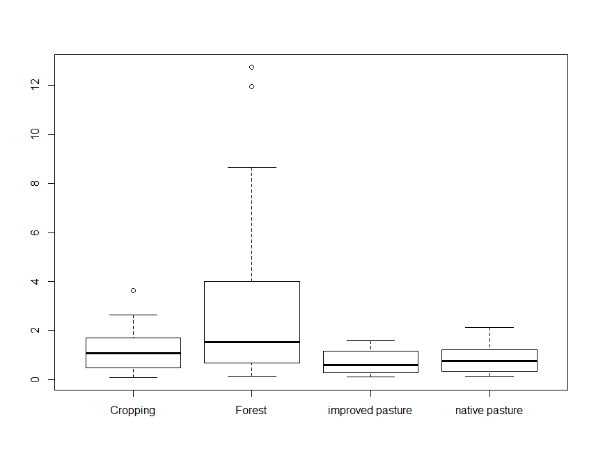
Note the use of the tilde symbol ∼ in the above command. The code
Total_Carbon∼Landclass is analogous to a model formula in this
case, and simply indicates that Total_Carbon is described by
Landclass and should be split up based on the category of this
variable. We will see more of this character with the specification of
soil spatial prediction functions later on.
Normal quantile and cumulative probability plots
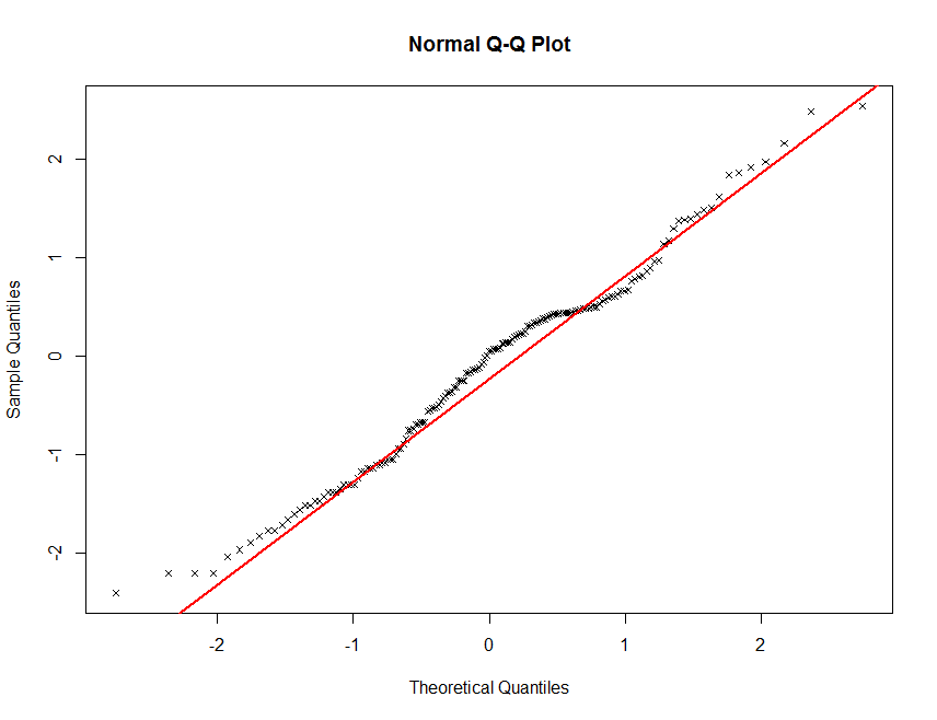
One way to assess the normality of the distribution of a given variable is with a quantile-quantile plot. This plot shows data values vs. quantiles based on a normal distribution.
    qqnorm(soil.data$Total_Carbon, plot.it = TRUE, pch = 4, cex = 0.7)
    qqline(soil.data$Total_Carbon, col = "red", lwd = 2)
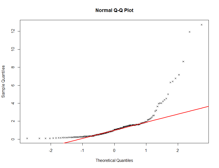
There definitely seems to be some deviation from normality here. This is not unusual for soil carbon information. It is common (in order to proceed with statistical modelling) to perform a transformation of sorts in order to get these data to conform to a normal distribution. Often a log transformation will be sutiable.
    qqnorm(log(soil.data$Total_Carbon), plot.it = TRUE, pch = 4, cex = 0.7)
    qqline(log(soil.data$Total_Carbon), col = "red", lwd = 2)
Finally, another useful data exploratory tool is quantile calculations.
R will return the quantiles of a given data set with the quantile
function. Note that there are nine different algorithms available for
doing this. You can find descriptions in the help file for quantile.
By default, the quartiles of a data distribution are given when using
this function, but any quantiles can be estimated using the probs
function parameter.
    quantile(soil.data$Total_Carbon, na.rm = TRUE)

    ##    0%   25%   50%   75%  100%
    ##  0.09  0.39  1.05  1.60 12.74

    quantile(soil.data$Total_Carbon, na.rm = TRUE, probs = seq(0, 1, 0.05))

    ##     0%     5%    10%    15%    20%    25%    30%    35%    40%    45%    50%
    ##  0.090  0.170  0.230  0.270  0.328  0.390  0.502  0.604  0.730  0.866  1.050
    ##    55%    60%    65%    70%    75%    80%    85%    90%    95%   100%
    ##  1.150  1.268  1.448  1.548  1.600  1.762  2.026  2.928  4.494 12.740

    quantile(soil.data$Total_Carbon, na.rm = TRUE, probs = seq(0.9, 1, 0.01))

    ##     90%     91%     92%     93%     94%     95%     96%     97%     98%     99%
    ##  2.9280  3.3208  3.9128  4.0152  4.2388  4.4940  5.5920  6.4488  7.0536  9.8344
    ##    100%
    ## 12.7400
Exercises
-
Using the
soil.dataset firstly determine the summary statistics for each of the numerical or quantitative variables. You want to calculate things like maximum, minimum, mean, median, standard deviation, and variance. There are a couple of ways to do this. However, put all the results into a data frame and export as a text file. -
Generate histograms and QQ plots for each of the quantitative variables. Do any need some sort of transformation so that their distribution is normal. If so, do the transformation and perform the plots again.