CODE:
Get the code used for this section here
Universal kriging prediction variance
- Defining the model parameters
- Mapping predictions and model uncertainties
- Evaluating the quantification of uncertainties
In the page regarding digital soil mapping of continuous variables, universal kriging was explored. This model is ideal from the perspective that both the correlated variables and model residuals are handled simultaneously. This model also automatically generates prediction uncertainty via the kriging variance. It is with this variance estimate that we can define a prediction interval. Here, a 90% prediction interval will be defined for the mapping purposes. Although for evaluation of the uncertainties, a number of levels of confidence will be defined and subsequently evaluated in order to assess the performance and sensitivity of the uncertainty estimates. This is done using the prediction interval coverage probability assessment.
Defining the model parameters
First we need to load in all the libraries that are necessary for this section and load in the necessary data, and prepare for the modeling work.
# load libraries
library(ithir)
library(sf)
library(terra)
library(gstat)

# point data
data(HV_subsoilpH)

# Start afresh round pH data to 2 decimal places
HV_subsoilpH$pH60_100cm <- round(HV_subsoilpH$pH60_100cm, 2)

# remove already intersected data
HV_subsoilpH <- HV_subsoilpH[, 1:3]

# add an id column
HV_subsoilpH$id <- seq(1, nrow(HV_subsoilpH), by = 1)

# re-arrange order of columns
HV_subsoilpH <- HV_subsoilpH[, c(4, 1, 2, 3)]

# Change names of coordinate columns
names(HV_subsoilpH)[2:3] <- c("x", "y")
# save a copy of coordinates
HV_subsoilpH$x2 <- HV_subsoilpH$x
HV_subsoilpH$y2 <- HV_subsoilpH$y

# convert data to sf object
HV_subsoilpH <- sf::st_as_sf(x = HV_subsoilpH, coords = c("x", "y"))

# grids (covariate rasters from ithir package)
hv.sub.rasters <- list.files(path = system.file("extdata/", package = "ithir"), pattern = "hunterCovariates_sub",
full.names = TRUE)

# read them into R as SpatRaster objects
hv.sub.rasters <- terra::rast(hv.sub.rasters)

# extract covariate data
DSM_data <- terra::extract(x = hv.sub.rasters, y = HV_subsoilpH, bind = T, method = "simple")
DSM_data <- as.data.frame(DSM_data)

# check for NA values
which(!complete.cases(DSM_data))

## integer(0)

DSM_data <- DSM_data[complete.cases(DSM_data), ]
Now to prepare the data for the universal kriging model. Below we partition the dataset via the randomized holdback routine whereby 70% of the data is used for model fitting work, leaving the other 30% for out-of-bag evaluation of the model plus the quantification of uncertainties.
# subset data for modeling
set.seed(123)
training <- sample(nrow(DSM_data), 0.7 * nrow(DSM_data))
DSM_data_cal <- DSM_data[training, ]
DSM_data_val <- DSM_data[-training, ]
The DSM_data_cal and DSM_data_val objects correspond to the model calibration and out-of-bag data sets respectively.
We will firstly use a step wise regression to determine a parsimonious model are the most important covariates.
## Linear regression model Full model
lm1 <- lm(pH60_100cm ~ Terrain_Ruggedness_Index + AACN + Landsat_Band1 + Elevation + Hillshading + Light_insolation + Mid_Slope_Positon + MRVBF + NDVI + TWI + Slope, data = DSM_data_cal)

# Parsimous model
lm2 <- step(lm1, direction = "both", trace = 0)
as.formula(lm2)

## pH60_100cm ~ Terrain_Ruggedness_Index + AACN + Landsat_Band1 +
##     Elevation + Hillshading + Light_insolation + Mid_Slope_Positon +
##     MRVBF + NDVI + TWI + Slope

summary(lm2)
Now we can construct the universal kriging model using the step wise selected covariates.
## Universal kriging model
names(DSM_data_cal)[3:4] <- c("x", "y")

# calculate empirical variogram
vgm1 <- variogram(pH60_100cm ~ Terrain_Ruggedness_Index + AACN + Landsat_Band1 +
Elevation + Hillshading + Light_insolation + Mid_Slope_Positon + MRVBF + NDVI +
TWI + Slope, ~x + y, data = DSM_data_cal, width = 200, cutoff = 3000)

# initialise variogram model parameters
mod <- vgm(psill = var(DSM_data_cal$pH60_100cm), "Sph", range = 3000, nugget = 0)

# fit model
model_1 <- fit.variogram(vgm1, mod)

# Universal kriging model object
gUK <- gstat(NULL, "hunterpH_UK", pH60_100cm ~ Terrain_Ruggedness_Index + AACN +
Landsat_Band1 + Elevation + Hillshading + Light_insolation + Mid_Slope_Positon +
MRVBF + NDVI + TWI + Slope, data = DSM_data_cal, locations = ~x + y, model = model_1)
gUK

## data:
## hunterpH_UK : formula = pH60_100cm`~`Terrain_Ruggedness_Index + AACN + Landsat_Band1 + Elevation + Hillshading + Light_insolation + Mid_Slope_Positon + MRVBF + NDVI + TWI + Slope ; data dim = 354 x 13
## variograms:
##                model     psill   range
## hunterpH_UK[1]   Nug 0.6391582   0.000
## hunterpH_UK[2]   Sph 0.6854493 565.514
## ~x + y
Mapping predictions and model uncertainties
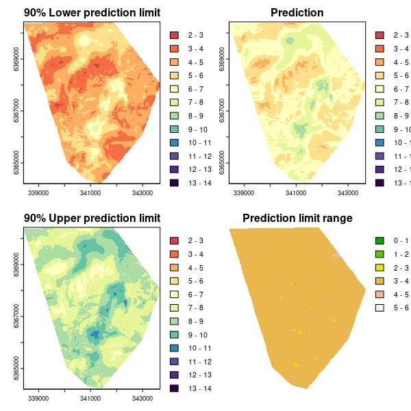
Here we want to produce four maps that will correspond to:
- The lower end of the 90% prediction interval or 5th percentile of the empirical probability density function.
- The universal kriging prediction.
- The upper end of the 90% prediction interval or 95th percentile of the empirical probability density function.
- The prediction interval range.
For the prediction we use the terra::interpolate function.
UK.P.maps <- terra::interpolate(object = hv.sub.rasters, model = gUK, xyOnly = FALSE)
The above generates 2 rasters, the first being the kriged prediction, the second being the kriging variance. Taking the square root of the kriging variance derives the standard deviation which we can then multiply by the quantile function value that corresponds either the lower (5th) or upper tail ((95th)) probability which is 1.644854. We then both add and subtract this value from the universal kriging prediction to derive the 90% prediction limits.
# standard deviation
f2 <- function(x) (sqrt(x))
UK.stdev.map <- terra::app(x = UK.P.maps[[2]], fun = f2)

# standard error
zlev <- qnorm(0.95)
f2 <- function(x) (x * zlev)
UK.mult.map <- terra::app(x = UK.stdev.map, fun = f2)

# Add and subtract standard error from prediction upper PL
UK.upper.map <- UK.P.maps[[1]] + UK.mult.map

# lower PL
UK.lower.map <- UK.P.maps[[1]] - UK.mult.map

# prediction range
UK.piRange.map <- UK.upper.map - UK.lower.map
So to plot them all together we use the following script. Here we explicitly create a color ramp that follows reasonably closely the pH color ramp. Then we scale each map to the common range for better comparison.
# color ramp
phCramp <- c("#d53e4f", "#f46d43", "#fdae61", "#fee08b", "#ffffbf", "#e6f598", "#abdda4", "#66c2a5", "#3288bd", "#5e4fa2", "#542788", "#2d004b")
brk <- c(2:14)

# plotting
par(mfrow = c(2, 2))
plot(UK.lower.map, main = "90% Lower prediction limit", breaks = brk, col = phCramp)
plot(UK.P.maps[[1]], main = "Prediction", breaks = brk, col = phCramp)
plot(UK.upper.map, main = "90% Upper prediction limit", breaks = brk, col = phCramp)
plot(UK.piRange.map, main = "Prediction limit range", col = terrain.colors(length(seq(0, 6.5, by = 1)) - 1), axes = FALSE, breaks = seq(0, 6.5, by = 1))
Evaluating the quantification of uncertainty
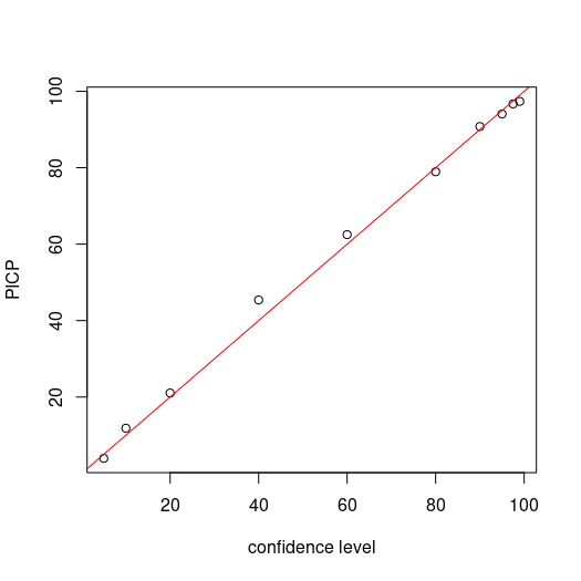
One of the ways to assess the performance of the uncertainty quantification is to evaluate the occurrence of times where an observed value is encapsulated by an associated prediction interval. Given a stated level of confidence, we should also expect to find the same percentage of observations encapsulated by its associated prediction interval. We define this percentage as the prediction interval coverage probability (PICP). The PICP was used in both Solomatine and Shrestha (2009) and Malone et al. (2011). To assess the sensitivity of the uncertainty quantification, we define prediction intervals at a number of levels of confidence and then assess the PICP. Ideally, a 1:1 relationship is expected.
First we apply the universal kriging model gUK to the out-of-bag data in order to estimate pH and the prediction variance.
names(DSM_data_val)[3:4] <- c("x", "y")
UK.preds.V <- krige(pH60_100cm ~ Terrain_Ruggedness_Index + AACN + Landsat_Band1 +
Elevation + Hillshading + Light_insolation + Mid_Slope_Positon + MRVBF + NDVI +
TWI + Slope, data = DSM_data_cal, locations = ~x + y, model = model_1, newdata = DSM_data_val)

# prediction standard deviation
UK.preds.V$stdev <- sqrt(UK.preds.V$var1.var)
Then we define a vector of quantile function values for a sequence of probabilities using the qnorm function.
# confidence levels
qp <- qnorm(c(0.995, 0.9875, 0.975, 0.95, 0.9, 0.8, 0.7, 0.6, 0.55, 0.525))
Then we estimate the prediction limits for each confidence level.
# standard error
vMat <- matrix(NA, nrow = nrow(UK.preds.V), ncol = length(qp))
for (i in 1:length(qp)) {
vMat[, i] <- UK.preds.V$stdev * qp[i]}

# upper
uMat <- matrix(NA, nrow = nrow(UK.preds.V), ncol = length(qp))
for (i in 1:length(qp)) {
uMat[, i] <- UK.preds.V$var1.pred + vMat[, i]}

# lower
lMat <- matrix(NA, nrow = nrow(UK.preds.V), ncol = length(qp))
for (i in 1:length(qp)) {
lMat[, i] <- UK.preds.V$var1.pred - vMat[, i]}
Then we want to evaluate the PICP for each confidence level.
## PICP
bMat <- matrix(NA, nrow = nrow(UK.preds.V), ncol = length(qp))
for (i in 1:ncol(bMat)) {
bMat[, i] <- as.numeric(DSM_data_val$pH60_100cm <= uMat[, i] &
DSM_data_val$pH60_100cm >= lMat[, i])}
Plotting the confidence level against the PICP provides a visual means to assess the fidelity about the 1:1 line. As can be seen below, the PICP follows closely the 1:1 line.
# make plot
par(mfrow = c(1, 1))
cs <- c(99, 97.5, 95, 90, 80, 60, 40, 20, 10, 5)
plot(cs, ((colSums(bMat)/nrow(bMat)) * 100), ylab = "PICP", xlab = "confidence level")
# draw 1:1 line
abline(a = 0, b = 1, col = "red")
So to summarize. We may evaluate the performance of the universal kriging model on the basis of the predictions. Using the out-of-bag data we would use the ithir::goof function for that purpose.
ithir::goof(observed = DSM_data_val$pH60_100cm, predicted = UK.preds.V$var1.pred)

##          R2 concordance      MSE     RMSE       bias
## 1 0.4263056   0.5714666 1.098039 1.047874 0.04732726
And then we may assess the uncertainties on the basis of the PICP like shown above, together with assessing the quantiles of the distribution of the prediction interval range for a given prediction confidence level (here 90%).
cs <- c(99, 97.5, 95, 90, 80, 60, 40, 20, 10, 5)  # confidence level
colnames(lMat) <- cs
colnames(uMat) <- cs
quantile(uMat[, "90"] - lMat[, "90"])

##       0%      25%      50%      75%     100%
## 2.857832 3.197809 3.358844 3.477724 3.902413
As can be noted above, the prediction interval range is relatively homogeneous and this is corroborated on the associated map created earlier.
References
Malone, B P, A B McBratney, and B Minasny. 2011. “Empirical Estimates of Uncertainty for Mapping Continuous Depth Functions of Soil Attributes.” Geoderma 160: 614–26.
Solomatine, D. P, and D. L Shrestha. 2009. “A Novel Method to Estimate Model Uncertainty Using Machine Learning Techniques.” Water Resources Research 45: Article Number: W00B11.