This poster “Managing quantifiable uncertainties in digital land suitability assessments” was on display at the Pedometrics 2017 conference held in Wageningen, The Netherlands.
Please read on if you more more information about the research that this poster summarizes. And don’t hesitate to leave some comments at the end.
Got here via QR Code?
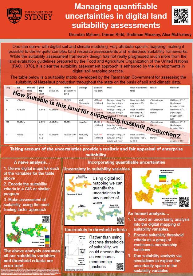
If you have gotten to this site via the QR code on the poster, please read the following description of how the figure showing the expected minimum suitability rating was created.
The short summary is that the map is an output of a land suitability analysis for hazelnuts across the Meander Valley irrigation area in north western Tasmania, Australia. Further contextual information about this area and land suitability analysis in general throughout Tasmania can be found here.
What is special about this map is that it is the result of incorporating all the quantified uncertainties that were derived for each of the suitability variables as summarized in the table matrix displayed at the top of the poster. The methods for quantifying the uncertainties of each of the variables is described in this paper. We also encoded the threshold criteria from the table into a set of continuous membership functions. The use of membership functions as an alternative to discrete threshold cutoffs recognizes that the absolute values used in the suitability analysis can be handled in a less strict manner. For example a discrete threshold of soil pH 5.5 could mean a soil is classified either as suitable or unsuitable if the site was 5.5 or 5.4 respectively. The use of continuous membership functions allows some wiggle room around this by expressing suitability as somewhere along a gradient between 0 and 1, with 1 being suitable and 0 being unsuitable. We may express the continuous memberships with a number of different functions to describe the relationship between the target variable characteristic and suitability. For example common membership functions include the parabolic function (which could be used to describe soil pH), the sigmoid function (could be used for soil depth perhaps), and the inverted sigmoid function (could be used for soil stoniness or conductivity). Or very simply the relationship could be expressed as a linear function. The poster shows the former 3 examples.
In the Malone et al. (2015) paper the analysis did not include the incorporation of membership functions for each of the hazelnut suitability variables. Nevertheless, the uncertainties of the variables themselves were handled by a simulation approach where with some clever re sampling approach we were able to generate different realizations of the variables and pass each one through an encoded representation of the suitability matrix table for hazelnuts. We generated many hundreds of realizations which when combined together allowed us the estimate the probability of whether each point on the mapping area was well suited, suited, moderately suited, or unsuited for hazelnut production. In the analysis conducted for this poster we included the continuous membership functions for each variable. Specifically these were:
- Soil depth. Sigmoid function. Soil depth was modeled in a two step process, such that soil depth was modeled as a binary variable to predict the occurrence of soils less than or equal to 50cm and soils greater than 50cm depth. With soils less than or equal to 50cm, an additional model step was implemented to predict the soil depth. The digital soil mapping steps were all conducted so that we could quantify the associated uncertainties. These uncertainties were considered in the ensuing suitability analysis. By observing the relationship of suitability and soil depth as summarized on the suitability matrix, it is clear that a sigmoid function would be appropriate here.
- Soil pH. Parabolic function
- Soil conductivity. Inverted sigmoid function
- Soil texture. Parabolic function
- Soil drainage. Sigmoid function
- Soil stoniness. Inverted sigmoid function. Like soil depth this variable was modelled in a two-step procedure. This included a model to predict the presence or absence of stones followed by a model where stones were present to predict the main size fraction.
- Frost. Inverted sigmoid function.
- Temperature. Parabolic function
- Rainfall (March). Inverted sigmoid function
Because the suitability analysis is no longer in the realm of designating a site to a specific class of suitability - as it is now expressed on a grading system due to the continuous membership function - it is slightly altered to what was conducted in Malone et al. (2015). The simulation approach still holds, however at each grid cell location, all the simulations are stacked for each variable before taking the average. We then take the minimum averaged membership probability between all suitability variables. This is equivalent to a most limiting factor approach, except we express it as the minimum probability found from each of the suitability variables at each grid cell location. Although not shown on the poster, with this approach we can also for each suitability variable, map the median and lower and upper prediction limits of the suitability analysis. We can also evaluate whether there may be multi-factor issues in relation to the suitability analysis. This is evaluated by working out the whether if more than one suitability variable has a rating of less than 50%.
Ultimately, while taking account of uncertainties in a digital land suitably assessment may change oftentimes optimistic outcomes as derived from an analysis that considers parameters to be error-free, it is important to conduct the analysis in a realistic and fair framework. This is one where we incorporate as best we can all the sources of uncertainty into the analysis. The approach described in Malone et al. (2015) and the additional analysis used in the research that is summarized in this poster is but one way of conducting a enterprise suitability analysis. There is likely to be simpler or more complex approaches that are very different to what was conducted here. We have just merely tried to advance the most-limiting factor approach to suitability analysis by framing it within a digital soil mapping approach where uncertainties can be explicitly defined.
Read on if you want to examine the conference abstract related to this poster.
Reference
Conference abstract
Authors: Brendan Malone, Darren Kidd, Budiman Minasny, Alex McBratney.
We are seeing an increasing activity in land resource assessments (LSA) at varying spatial scales throughout the world. These efforts have been largely assisted by suites of digital information technologies such as digital soil and climate modeling and mapping, and associated environmental resource mapping such as remote sensing data and digital elevation models. A common scenario however is that these digital LSAs are made with the assumption that the input information is error free. Similarly, the criteria with which assessments are made are often discretely defined.
In this paper we briefly review the status quo of digital land suitability analysis. The study then focuses on Tasmania, Australia where there has been the integration within Government policy and directives, a fully digital LSA system for a number of specific agricultural enterprises. Here we address two issues that present limitations to current LSAs. First we take into account the quantified uncertainties of the input variables. Secondly, we adopt membership functions rather than discrete threshold values for the assessment criteria.
For taking into account the input variable uncertainties, simulations are used to generate plausible realizations of soil and climatic variables for input into an LSA. It is found that when comparing to a LSA that assumes inputs to be error free, there is a significant difference in the assessment of suitability. Using an approach that assumes inputs to be error free, 56% of the selected study area was predicted to be suitable for hazelnuts (our selected agricultural enterprise). Using the simulation approach it is revealed that there is considerable uncertainty about the ‘error free’ assessment, where a prediction of ‘unsuitable’ was made 66% of the time (on average) at each grid cell of the study area. In the specific case of our study area, the cause of this difference is that digital soil mapping of both soil pH and conductivity have a high quantified uncertainty in this study area. The use of parameter membership functions and or adopting expert rules around soil properties that can be easily managed, we find penalties for taking into account uncertainties are not as severe. Despite differences between the comparative methods, taking account of the prediction uncertainties provide a realistic appraisal of enterprise suitability. It is advantageous also because suitability assessments are provided as continuous variables as opposed to discrete classifications. We would recommend for other studies that consider similar FAO (Food and Agriculture Organisation of the United Nations) land evaluation framework type suitability assessments, that parameter membership functions together with the simulation approach are used in concert.
Further information
The naive analysis that was conducted for this poster has been summarised and coded in R in the Using R for Digital Soil Mapping book.
While a bit messy, the underlying code for conducting the suitability analysis can be found at this Bitbucket Repo.
The repo scripts conduct 3 main tasks:
- A Naive analysis that considers inputs to be error free
- An analysis that takes into consideration the underlying uncertainties of the input variables. This approach is described in Malone et al. (2015)
- An extension of the Malone et al. (2015) approach that considers the suitability threshold criteria as continuous membership functions.