CODE:
Get the code used for this section here
Example of two-step digital soil mapping
- Pre-reading background
- Data preparation
- Two-stage model fitting and evaluation
- Model for predicting horizon occurence
- Soil profile reconstructions
- Spatial extension of the two-stage soil horizon occurrence and depth model
Pre-reading background
The motivation for this section is to gain some insights into a digital soil mapping approach that uses a combination of both continuous and categorical attribute modeling. Subsequently, we will build on the efforts of the training materials that dealt with each of these type of modeling approaches separately.
There are some situations where, a combinatorial modeling approach might be suitable in a digital soil mapping work flow. An example of such a workflow is in Malone et al. (2015) in regards to the prediction of soil thickness. The context behind that approach was that often lithic contact was not achieved during the soil survey activities, effectively indicating soil depth was greater than the soil probing depth (which was 1.5 m). Where lithic contact was found, the resulting depth was recorded. The difficulty in using this data in the raw form was that there were many sites where soil depth was greater than 1.5 m together with actual recorded soil depth measurements. The nature of this type of data is likened to a zero-inflated distribution, where many zero observations are recorded among actual measurements (Sileshi 2008).
In Malone et al. (2015) the zero observations were attributed to soil depth being greater than 1.5m. They therefore performed the modeling in two stages. First modeling involved a categorical or binomial model of soil depth being greater than 1.5 m or not. This was followed by continuous attribute modeling of soil depth using the observations where lithic contact was recorded. While the approach was a reasonable solution, it may be the case that the frequency of recorded measurements is low, meaning that the spatial modeling of the continuous attribute is made under considerable uncertainty, as was the case in Malone et al. (2015) with soil depth and other environmental variables spatially modeled in that study; for example, the frequency of winter frosts.
Another interesting example of a combinatorial DSM work flow was
described in Gastaldi et al. (2012) for the mapping of
occurrence and thickness of soil horizons. There they used a multinomial
logistic model to predict the presence or absence of the given soil
horizon class, followed by continuous attribute modeling of the horizon
depths. For the purposes a demonstrating the work flow of this
combinatorial or two-stage DSM, we will re-visit the approach that is
described by Gastaldi et al. (2012) and work through
the various steps needed to perform it within R.
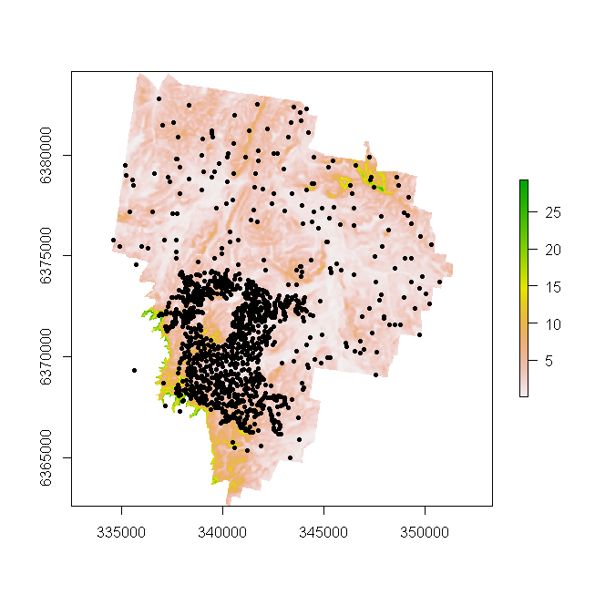
The data we will use comes from 1342 soil profile and core descriptions from the Lower Hunter Valley, NSW Australia. These data have been collected on an annual basis since 2001 to present. These data are distributed across the 220km2 area as shown in Figure below. The intention is to use these data first to predict the occurrence of given soil horizon classes (following the nomenclature of the Australian Soil Classification (Isbell 2002). Specifically we want to prediction the spatial distribution of the occurrence of A1, A2, AP, B1, B21, B22, B23, B24, BC, and C horizons, and then where those horizons occur, predict their depth.
Data preparation
First lets perform some data discovery both in terms of the soil profile data and spatial covariates to be used as predictor variables and to inform the spatial mapping.
The point data used for this exercise can be downloaded from here
and then loaded into the R environment as below.
You will notice the soil profile data datis arranged in a flat file
where each row is a soil profile. There are many columns of information
which include profile identifier and spatial coordinates. Then there are
11 further columns that are binary indicators of whether a horizon class
is present or not (indicated as 1 and 0 respectively). The following
11 columns after the binary columns indicate the horizon depth for the
given horizon class.
# load libraries that are used in this exercise
library(ithir)
library(sf)
library(terra)
library(aqp)
library(nnet)
library(MASS)
library(quantregForest)

# data
load("HV_horizons.rda")
str(dat)

## 'data.frame':    1342 obs. of  25 variables:
##  $ FID : Factor w/ 1342 levels "1","10","100",..: 1 2 3 4 5 6 7 8 9 10 ...
##  $ e   : num  338014 338183 341609 341352 339736 ...
##  $ n   : num  6370646 6370550 6370437 6370447 6370439 ...
##  $ A1  : int  1 0 1 1 1 1 1 0 1 1 ...
##  $ A2  : int  1 0 0 0 0 1 1 0 0 0 ...
##  $ AP  : int  0 1 0 0 0 0 0 1 0 0 ...
##  $ B1  : int  0 0 1 1 1 0 0 0 1 0 ...
##  $ B21 : int  1 1 1 1 1 1 1 1 1 1 ...
##  $ B22 : int  1 0 1 0 1 1 1 1 1 1 ...
##  $ B23 : int  0 0 0 0 0 0 0 0 0 0 ...
##  $ B24 : int  0 0 0 0 0 0 0 0 0 0 ...
##  $ B3  : int  0 0 0 0 0 0 0 0 0 0 ...
##  $ BC  : int  0 0 0 0 0 0 0 0 1 1 ...
##  $ C   : int  0 0 0 0 0 0 0 0 0 0 ...
##  $ A1d : num  21 NA 17 45 20 25 13 NA 10 44 ...
##  $ A2d : num  27 NA NA NA NA 15 13 NA NA NA ...
##  $ APd : num  NA 40 NA NA NA NA NA 35 NA NA ...
##  $ B1d : num  NA NA 25 25 30 NA NA NA 30 NA ...
##  $ B21d: num  26 60 26 30 30 25 58 40 20 38 ...
##  $ B22d: num  26 NA 32 NA 20 20 16 25 25 18 ...
##  $ B23d: int  NA NA NA NA NA NA NA NA NA NA ...
##  $ B24d: int  NA NA NA NA NA NA NA NA NA NA ...
##  $ B3d : int  NA NA NA NA NA NA NA NA NA NA ...
##  $ BCd : int  NA NA NA NA NA NA NA NA 15 NA ...
##  $ Cd  : int  NA NA NA NA NA NA NA NA NA NA ...

# Change cases of very thin A1 horizons to having no A1 horizon needed for
# purposes of demonstrating workflow rather than advancing scientific inquiry
dat$A1[dat$A1d <= 15] <- 0

# convert point to spatial object
dat <- sf::st_as_sf(x = dat, coords = c("e", "n"))
At our disposal are several covariates that have been derived entirely
from a digital elevation model. These data are available from the
ithir package and can be loaded as below.
# grids (covariate rasters from ithir package)
hv.rasters <- list.files(path = system.file("extdata/", package = "ithir"), pattern = "hunterCovariates_A", full.names = T)

# read them into R as SpatRaster objects
hv.rasters <- terra::rast(hv.rasters)
## raster properties
hv.rasters

## class       : SpatRaster
## dimensions  : 860, 675, 8  (nrow, ncol, nlyr)
## resolution  : 25, 25  (x, y)
## extent      : 334497.3, 351372.3, 6362628, 6384128  (xmin, xmax, ymin, ymax)
## coord. ref. :
## sources     : hunterCovariates_A_AACN.tif
##               hunterCovariates_A_elevation.tif
##               hunterCovariates_A_Hillshading.tif
##               ... and 5 more source(s)
## names       : hunte~_AACN, hunte~ation, hunte~ading, hunte~ation, hunte~MRVBF, hunte~Slope, ...
## min values  :      0.0000,     27.3035,      0.0000,    988.5308,    0.000000,     0.00100, ...
## max values  :    211.1496,    322.1442,     62.6977,   1969.7966,    6.975086,    36.21008, ...
For a quick check, lets overlay the soil profile points onto the DEM. You will notice on the Figure below the area of concentrated soil survey (which represents locations of annual survey) within the extent of a regional scale soil survey across the whole study area.
## Overlay points onto raster
plot(hv.rasters[[2]])
points(dat, pch = 20)
The last preparatory step we need to take is the covariate intersection of the soil profile data, and remove any sites that are outside the mapping extent or simply do not have the full complement of covariate data.
# Covariate extract for points
ext <- terra::extract(x = hv.rasters, y = dat, bind = T, method = "simple")
dsm.dat <- as.data.frame(ext)

# remove sites with missing covariates
dsm.dat <- dsm.dat[complete.cases(dsm.dat[, 24:31]), ]
Two-stage model fitting and evaluation
The two-stage modeling work flow for the A1 horizon modelling is stepped through below. This process would be repeated for the other horizon occurrences and their thicknesses. Some model evaluations and model outcomes will be provided below to advance the general discussion and assess how outputs might be combined to look at full soil profiles and their horizon compositions. Moreover, the applicability the estimated soil profile compositions can also be compared against their observed counterparts for the purposes of evaluation.
First we want to subset 75% of the data for calibrating models, and keeping the rest aside for out-of-bag model evaluation.
## Set target variable and subset data for validation A1 Horizon
dsm.dat$A1 <- as.factor(dsm.dat$A1)
summary(dsm.dat$A1)

##   0   1
## 712 619

# random subset
set.seed(123)
training <- sample(nrow(dsm.dat), 0.75 * nrow(dsm.dat))
# calibration dataset
dsm.cal <- dsm.dat[training, ]
# out-of-bag model evaluation data
dsm.val <- dsm.dat[-training, ]
Model for predicting horizon occurence
We first want to model the presence/absence in this case of the A1 horizon. We will use a multinomial model, followed up with a stepwise regression procedure in order to remove potentially redundant predictor variables.
# A1 presence or absence model
mn1 <- nnet::multinom(formula = A1 ~ hunterCovariates_A_AACN + hunterCovariates_A_elevation + hunterCovariates_A_Hillshading + hunterCovariates_A_light_insolation + hunterCovariates_A_MRVBF + hunterCovariates_A_Slope + hunterCovariates_A_TRI + hunterCovariates_A_TWI, data = dsm.cal)

# stepwise variable selection
mn2 <- stepAIC(mn1, direction = "both", trace = FALSE)

summary(mn2)

## Call:
## nnet::multinom(formula = A1 ~ hunterCovariates_A_elevation +
##     hunterCovariates_A_MRVBF, data = dsm.cal)
##
## Coefficients:
##                                    Values   Std. Err.
## (Intercept)                  -0.880315066 0.308536659
## hunterCovariates_A_elevation  0.004513106 0.002350626
## hunterCovariates_A_MRVBF      0.175753835 0.054693734
##
## Residual Deviance: 1366.553
## AIC: 1372.553
We use the goofcat function from ithir to evaluate the model quality
both in terms of the calibration and out-of-bag data.
## model Goodness of fit calibration
mod.pred <- predict(mn2, newdata = dsm.cal, type = "class")
goofcat(observed = dsm.cal$A1, predicted = mod.pred)

## $confusion_matrix
##     0   1
## 0 441 347
## 1  98 112
##
## $overall_accuracy
## [1] 56
##
## $producers_accuracy
##  0  1
## 82 25
##
## $users_accuracy
##  0  1
## 56 54
##
## $kappa
## [1] 0.06479926

# validation
val.pred <- predict(mn2, newdata = dsm.val, type = "class")
goofcat(observed = dsm.val$A1, predicted = val.pred)

## $confusion_matrix
##     0   1
## 0 143 117
## 1  30  43
##
## $overall_accuracy
## [1] 56
##
## $producers_accuracy
##  0  1
## 83 27
##
## $users_accuracy
##  0  1
## 56 59
##
## $kappa
## [1] 0.097328
It is clear that the mn2 model appears to be moderately effective to
distinguish sites where the A1 horizon is absent with the given data and
predictive covariates.
Model for predicting horizon thickness
What we want to do now is to model the A1 horizon depth.
We will be using an alternative model to those that have been examined in this book so far. The is a quantile regression forest, which is a generalized implementation of the random forest model from Breiman (2001).
The algorithm is available via the quantregForest package, and further
details about the model can be found at Meinshausen (2006). The caret
package also interfaces with this model too.
Fundamentally, random forests are integral to the quantile regression algorithm. However, the useful feature and advancement from normal random forests is the ability to infer the full conditional distribution of a response variable. This facility is useful for building non-parametric prediction intervals for any given level of confidence information and also the ability to detect outliers in the data easily.
Quantile regression used via the quanregForest algorithm is
implemented in the chapter simply to demonstrate the wide availability
of prediction models and machine learning methods that can be used in
digital soil mapping.
Getting the model initiated we first need to perform some preparatory
tasks. Namely the removal of missing data from the available data set
i.e those cases where no A1 horizon exists as the horizon thickness data
is currently give the value NA.
# Remove missing values calibration
mod.dat <- dsm.cal[!is.na(dsm.cal$A1d), ]

# out of bag cases
val.dat <- dsm.val[!is.na(dsm.val$A1d), ]
It is useful to check the inputs required for the quantile regression forests (using the help file); however its parameterization is largely similar to other models that have been used already in this book, particularly those for the random forest models.
# Fit quantile regression forest model
qrf <- quantregForest(x = mod.dat[, 24:31], y = mod.dat$A1d, importance = TRUE)
qrf

##
##  Call:
##  quantregForest(x = mod.dat[, 24:31], y = mod.dat$A1d, importance = TRUE)
##
##                      Number of trees: 500
## No. of variables tried at each split: 2

# variable importances
importance(qrf)

##                                       %IncMSE IncNodePurity
## hunterCovariates_A_AACN              6.626844      12234.84
## hunterCovariates_A_elevation        14.208151      12891.47
## hunterCovariates_A_Hillshading      15.045393      10780.55
## hunterCovariates_A_light_insolation  8.411560      12251.45
## hunterCovariates_A_MRVBF            16.520712      13731.85
## hunterCovariates_A_Slope            13.848516      10840.27
## hunterCovariates_A_TRI              17.047087      11984.96
## hunterCovariates_A_TWI               7.802111      11952.38
Naturally, the best test of the model is to evaluate it against out-of-bag cases. In addition to our normal validation procedure we can also derive the PICP for the validation data too.
## model Goodness of fit Calibration
quant.cal <- predict(qrf, newdata = mod.dat[, 24:31], all = T)
goof(observed = mod.dat$A1d, predicted = quant.cal[, 2], plot.it = T)

##          R2 concordance      MSE     RMSE       bias
## 1 0.8969432   0.9040645 18.42857 4.292851 -0.7730415

# out of bag cases
quant.val <- predict(qrf, newdata = val.dat[, 24:31], all = T)
goof(observed = val.dat$A1d, predicted = quant.val[, 2], plot.it = T)

##           R2 concordance     MSE     RMSE      bias
## 1 0.03717959  0.08385013 156.605 12.51419 -3.398577

# Prediction interval coverage probability
sum(quant.val[, 1] <= val.dat$A1d & quant.val[, 2] >= val.dat$A1d)/nrow(val.dat)

## [1] 0.366548
Based on the outputs above, the calibration model seems a reasonable outcome for the model, but is proven to be considerably overfitted when it is evaluated aginst the out-of-bag cases. We should also be expecting a PICP close to 90%, but this is clearly not the case above.
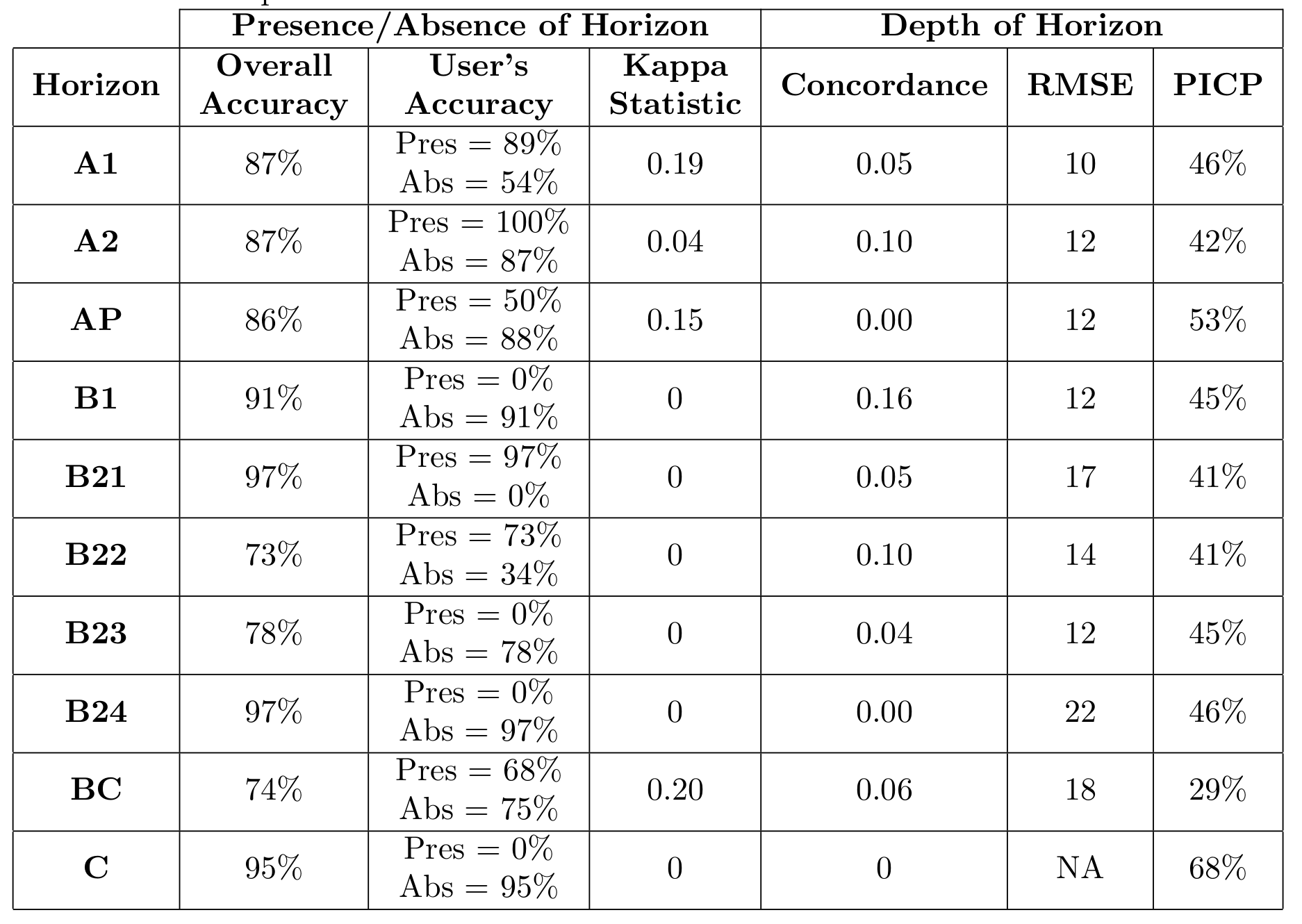
What has been covered above for the two-stage modeling is repeated for all the other soil horizons, with the main results displayed in the Table below. These statistics are reported based on the out-of-bag data.
It clear that there is a considerable amount of uncertainty overall in the various soil horizon models. For some horizons the results are a little encouraging; for example the model to predict the presence of a BC horizon is quite good. It is clear however that distinguishing between different B2 horizons is challenging. However predicting the presence or absence of a B22 horizons seems acceptable.
Soil profile reconstructions
Another way to assess the quality of the two-stage modeling is to assess first the number of soil profile that have matching sequences of soil horizon types. The following are two associated data sets. The firstare out-of-bag observed soil profiles with their horizon designations and associated thicknesses. The other are the corresponding profiles that have been predicted using the above two-step modeling processes.
# observed soil profiles
obs.profs <- read.table(file = "validation_obs.txt", sep = ",", header = T)

# associated predicted soil profiles
pred.profs <- read.table(file = "validation_outs.txt", sep = ",", header = T)
Below we can compare row for row the observed vs. the predicted in very
much a manual way. Using the match function we can quantify horizon
and horizon matches, or as below full sol profile soil horizon sequence
matching.
# Validation data horizon observations (1st 3 rows)
obs.profs[1:3, c(1, 4:14)]

##    FID A1 A2 AP B1 B21 B22 B23 B24 B3 BC C
## 1  101  1  0  0  1   1   0   0   0  0  0 0
## 2 1022  0  0  1  0   1   1   0   0  0  0 0
## 3 1026  1  0  0  0   1   1   0   0  0  0 0

# Associated model predictions (1st 3 rows)
pred.profs[1:3, 1:12]

##   dat.V.FID a1 a2 ap b1 b21 b22 b23 b24 b3 bc c
## 1       101  1  0  0  0   1   1   0   0  0  0 0
## 2      1022  1  0  0  0   1   1   0   0  0  0 0
## 3      1026  1  0  0  0   1   1   0   0  0  0 0

# matched soil profiles
sum(obs.profs$A1 == pred.profs$a1 & obs.profs$A2 == pred.profs$a2 & obs.profs$AP ==
pred.profs$ap & obs.profs$B1 == pred.profs$b1 & obs.profs$B21 == pred.profs$b21 &
obs.profs$B22 == pred.profs$b22 & obs.profs$B23 == pred.profs$b23 & obs.profs$B24 == pred.profs$b24 & obs.profs$B3 == pred.profs$b3 & obs.profs$BC == pred.profs$bc & obs.profs$C == pred.profs$c)/nrow(obs.profs)

## [1] 0.2222222
The result above indicates that just over 20% of soil profiles have
matched sequences of horizons. We can examine visually a few of these
matched profiles to examine whether there is much coherence in terms of
observed and associated predicted horizon depths. We will select out two
soil profiles: One with an AP horizon, and the other with an A1 horizon.
We can demonstrate this using the aqp package, which is a dedicated
R package for handling soil profile data collections.
# Subset of matching data (observations)
match.dat <- obs.profs[which(obs.profs$A1 == pred.profs$a1 & obs.profs$A2 == pred.profs$a2 & obs.profs$AP == pred.profs$ap & obs.profs$B1 == pred.profs$b1 & obs.profs$B21 == pred.profs$b21 & obs.profs$B22 == pred.profs$b22 & obs.profs$B23 == pred.profs$b23 & obs.profs$B24 == pred.profs$b24 & obs.profs$B3 == pred.profs$b3 & obs.profs$BC == pred.profs$bc & obs.profs$C == pred.profs$c), ]

# Subset of matching data (predictions)
match.dat.P <- pred.profs[which(obs.profs$A1 == pred.profs$a1 & obs.profs$A2 == pred.profs$a2 & obs.profs$AP == pred.profs$ap & obs.profs$B1 == pred.profs$b1 & obs.profs$B21 == pred.profs$b21 & obs.profs$B22 == pred.profs$b22 & obs.profs$B23 == pred.profs$b23 & obs.profs$B24 == pred.profs$b24 & obs.profs$B3 == pred.profs$b3 & obs.profs$BC == pred.profs$bc & obs.profs$C == pred.profs$c), ]
Now we just select any row where we know there is and AP horizon
match.dat[49, ]  #observation

##     FID      e       n A1 A2 AP B1 B21 B22 B23 B24 B3 BC C A1d A2d APd B1d B21d
## 195 642 338096 6372259  0  0  1  0   1   1   0   0  0  1 0  NA  NA  10  NA   30
##     B22d B23d B24d B3d BCd

match.dat.P[49, ]  #prediction

##     dat.V.FID a1 a2 ap b1 b21 b22 b23 b24 b3 bc c a1d a2d      apd b1.1 b21d
## 195       642  0  0  1  0   1   1   0   0  0  1 0  18  16 21.92308   18   31
##     b22d b23d     b24d b3d bcd cd
## 195   27   20 15.41176  NA  32 NA
We can see in these two profiles, the sequence of horizons is AP, B21, B22, BC. Now we just need to upgrade the data to a soil profile collection.
Using the horizon classes together with the associated depths, we want
to plot both soil profiles for comparison. First we need to create a
data frame of the relevant data then upgrade to a
soilProfileCollection, then finally plot.
The script below demonstrates this for the soil profile with the AP horizon. The same can be done with the associated soil profile with the A1 horizon. The plot of the is shown in the Figure below.
# Horizon classes
H1 <- c("AP", "B21", "B22", "BC")

# Extract horizon depths then combine to create soil profiles
p1 <- c(22, 31, 27, 32)
p2 <- c(10, 30, 15, 45)
p1u <- c(0, (0 + p1[1]), (0 + p1[1] + p1[2]), (0 + p1[1] + p1[2] + p1[3]))
p1l <- c(p1[1], (p1[1] + p1[2]), (p1[1] + p1[2] + p1[3]), (p1[1] + p1[2] + p1[3] + p1[4]))
p2u <- c(0, (0 + p2[1]), (+p2[1] + p2[2]), (+p2[1] + p2[2] + p2[3]))
p2l <- c(p2[1], (p2[1] + p2[2]), (p2[1] + p2[2] + p2[3]), (p2[1] + p2[2] + p2[3] +
p2[4]))

# Upper depths
U1 <- c(p1u, p2u)
# Lower depths
L1 <- c(p1l, p2l)

# Soil profile names
S1 <- c("predicted profile", "predicted profile", "predicted profile", "predicted profile", "observed profile", "observed profile", "observed profile", "observed profile")

# Random soil colors selected to distinguish between horizons
hue <- c("10YR", "10R", "10R", "10R", "10YR", "10R", "10R", "10R")
val <- c(4, 5, 7, 6, 4, 5, 7, 6)
chr <- c(3, 8, 8, 1, 3, 8, 8, 1)

# Combine all the data
TT1 <- data.frame(S1, U1, L1, H1, hue, val, chr)

# Convert munsell colors to rgb
TT1$soil_color <- with(TT1, munsell2rgb(hue, val, chr))

# Upgrade to soil profile collection
aqp::depths(TT1) <- S1 ~ U1 + L1

# Plot observed and associated predicted soil profiles
plot(TT1, name = "H1", colors = "soil_color")
title("Selected soil with AP horizon", cex.main = 0.75)
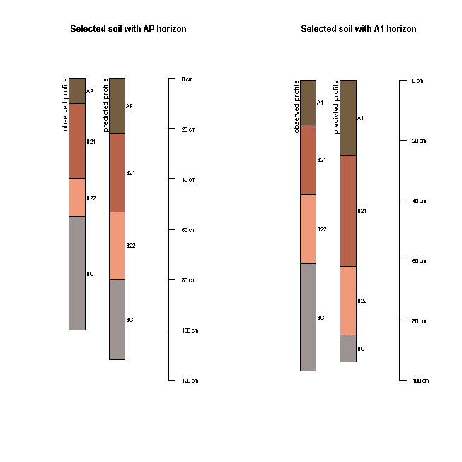
Soil is very complex, and while there is a general agreement between observed and associated predicted soil profiles, the power of the models used in this two-stage example has certainly been challenged. Recreating the arrangement of soil horizons together with maintenance of their depth properties is an interesting problem for pedometric studies and one that is likely to be pursued with vigor as better methods become available.
Spatial extension of the two-stage soil horizon occurrence and depth model
We will recall from previous chapters the process for applying prediction models across a mapping extent.
In the case of the two-stage model the mapping work flow if first creating the map of horizon presence/occurrence.
Then we apply the horizon depth model.
In order to ensure that the depth model is not applied to the areas where a particular soil horizon is predicted as being absent, those areas are masked out.
Maps for the presence of the A1 and AP horizons and their respective depths are displayed in the Figure below. The following scripts show the process of applying the two-stage model for the A1 horizon.
## MAPPING Apply A1 horizon presence/absence model spatially
A1.class <- terra::predict(object = hv.rasters, model = mn2)
A1.class
plot(A1.class, main = "A1-horizon occurence")

# Apply A1 horizon depth model spatially get covariates into a table
tempD <- data.frame(cellNos = seq(1:terra::ncell(hv.rasters)))
vals <- as.data.frame(terra::values(hv.rasters))
tempD <- cbind(tempD, vals)
tempD <- tempD[complete.cases(tempD), ]
cellNos <- c(tempD$cellNos)
gXY <- data.frame(terra::xyFromCell(hv.rasters, cellNos))
tempD <- cbind(gXY, tempD)
str(tempD)

# extend model to covariates
A1.depth <- predict(newdata = tempD, object = qrf)
# append coordinates
A1.depth.map <- cbind(data.frame(tempD[, c("x", "y")]), A1.depth)
# create raster
A1.depth.map <- terra::rast(x = A1.depth.map[, c(1, 2, 4)], type = "xyz")
plot(A1.depth.map, main = "A1-horizon thickness (unmasked)")

# Mask out areas where horizon is absent
msk <- terra::ifel(A1.class != 1, NA, 1)
plot(msk)
A1.depth.masked <- terra::mask(A1.depth.map, msk, inverse = T)
plot(A1.depth.masked, main = "A1-horizon thickness (masked)")
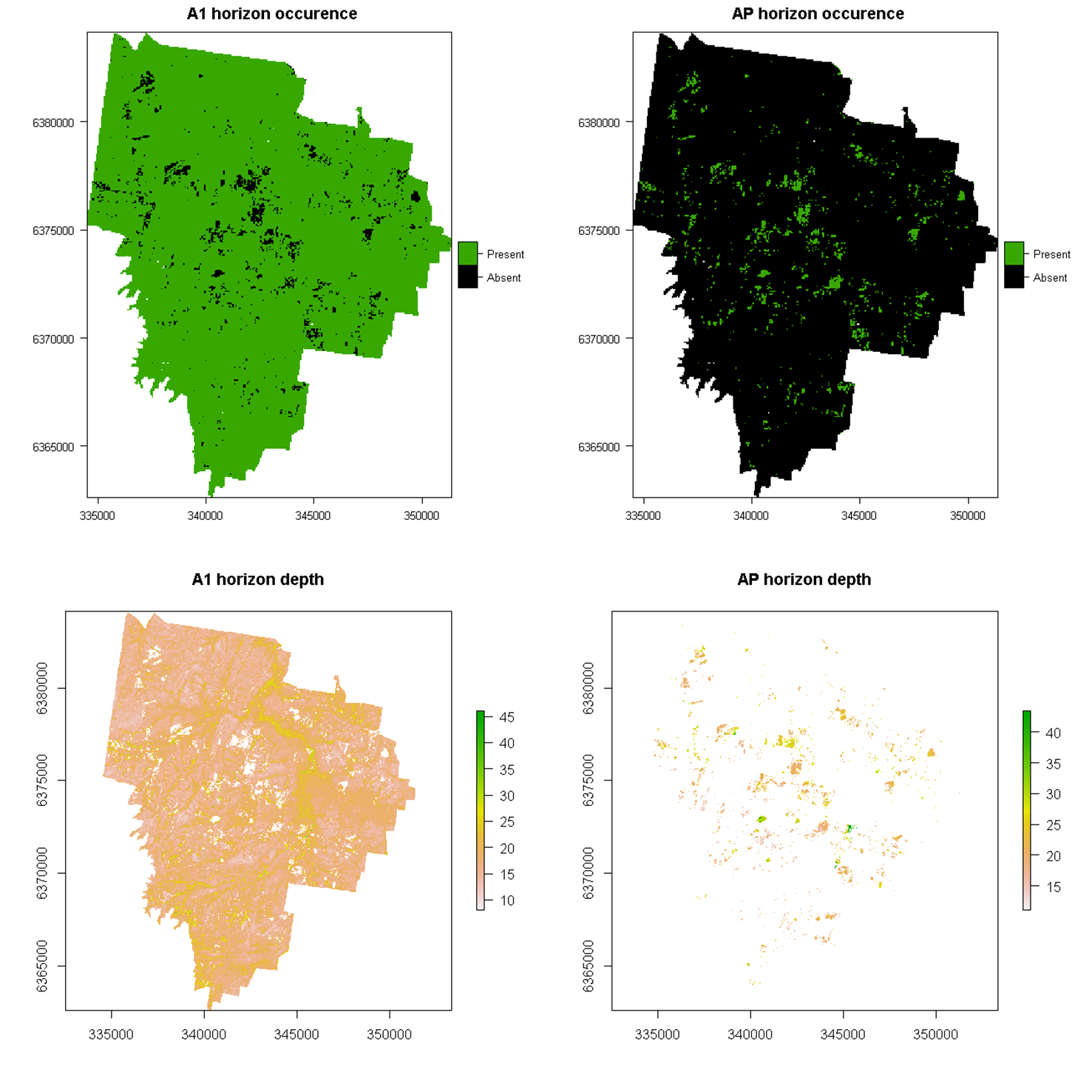
This figure displays an interesting pattern whereby AP horizons occur where A1 horizons do not. This makes reasonable sense. The spatial pattern of the AP horizon coincides generally with the distribution of vineyards across the study area, where soils are often cultivated and consequently removing the presence of the A1 horizon. Increased depth of A1 horizons also appears to be the case too in lower lying and stream channel catchments of the study area.
References
Breiman, L. 2001. “Random Forests.” Machine Learning 41: 5–32.
Gastaldi, G., Budiman Minasny, and Alex B. McBratney. 2012. “Mapping the Occurrence and Thickness of Soil Horizons.” Edited by Budiman Minasny, Brendan P. Malone, and Alex B. McBratney. London: Taylor & Francis.
Isbell, R. F. 2002. The Australian Soil Classification: Revised Edition. Collingwood, VIC: CSIRO Publishing.
Malone, Brendan P., Darren B. Kidd, Budiman Minasny, and Alex B. McBratney. 2015. “Taking Account of Uncertainties in Digital Land Suitability Assessment.” PeerJ, 3:e1366.
Meinshausen, Nicolai. 2006. “Quantile Regression Forests.” Journal of Machine Learning Research 7: 983–99.
Sileshi, Gudeta. 2008. “The Excess-Zero Problem in Soil Animal Count Data and Choice of Appropriate Models for Statistical Inference.” Pedobiologia 52 (1): 1–17. https://doi.org/http://dx.doi.org/10.1016/j.pedobi.2007.11.003.