CODE:
Get the code used in this section on cross-validation strategies
Cross-validation strategies
On the goodness of fit page we performed an evaluation of the mod.1 model which was a regression to predict soil CEC from clay content.
Usually it is more appropriate to evaluate a model using data that was not included for model fitting. Model evaluation has a few different forms and we will cover the main ones on this page.
Background notes
For completely unbiased assessments of model quality, it is ideal to have an additional data set that is completely independent of the model data.
When we are validating trained models with some sort of data sub-setting mechanism, always keep in mind that the validation statistics will be biased. As Brus et al. (2011) explains, the sampling from the target mapping area to be used for DSM is more-often-than-not from legacy soil survey, that in general would not have been based on some sort of probability sampling design. Therefore, that sample will be biased i.e not a true representation of the total population.
Even though we may randomly select observations from the legacy soil survey sites, those validation points do not become a probability sample of the target area, and consequently will only provide biased estimates of model quality.
Thus an independent probability sample is required. Further ideas on the statistical evaluation of models can be found in Hastie et al. (2001). It is recommended that some flavor of random sampling from the target area be conducted, to which there are a few types such as simple random sampling and stratified simple random sampling. Further information regarding sampling, sampling designs, their formulation and the relative advantages and constraints of each are described in Gruijter et al. (2006).
Usually from an operational perspective it is difficult to arrange the additional costs of organizing and implementing some sort of probability sampling for determining unbiased model quality assessment. The alternative is to perform some sort of data sub-setting, such that with a dataset, we split it into a set for model calibration and another set for evaluation.
This type of procedure can take different forms: the two main ones being random-hold back and leave-one-out-cross-validation (LOCV).
Random-hold back (or sometimes k-fold validation) is where we may sample a data set of some pre-determined proportion (say 70%) for which is used for model calibration. We then validate the model using the other 30% of the data. This is usually done using sampling without replacement which is when a case has been selected, it is never offered up for sampling again. The alternative is sampling with replacement which is where a sample that has been selected is again put back into the main set, making it possible for this same case be sampled again.
Sampling with replacement does not change the underlying probabilities that a case will be sampled. This is not the case for sampling without replacement.
Bootstrapping is the common term to describe the sampling technique (sampling with replacement) where the number of samples taken from the dataset equals the number of cases in the data. Evidently, about 63% of unique data cases are captured in this sample (Efron and Tibshirani 1997), leaving behind the other 37% of data cases for model evaluation.
For k-fold validation we divide the data set into equal sized partitions or folds, with all but one of the folds being used for the model calibration, the remaining fold is used for validation.
Like any other the other cross-validation strategies, we could repeat this k-fold process a number of times, each time using a different random sample from the data set for model calibration and evaluation. This allows one to efficiently derive distributions of the model evaluation statistics as a means of assessing the stability and sensitivity of the models and parameters.
A variant of the k-fold cross-validation is spatial cross-validation (Lovelace, Nowosad, and Muenchow 2019) where instead of random subsets of data to act as the different folds, the data are clustered spatially into groups (which we can think of as folds to keep with the general idea). Randomly splitting spatial data can lead to training points that are neighbors in space with test points. Due to spatial autocorrelation there is a chance the calibration and validation datasets may not be independent, with the consequence that CV fails to detect a possible overfitting. We will explore spatial cross-validation once we start usng spatial data in further exercises.
For now lets just focus on conventional CV techniques to bed done some fundamental concepts. You may note the some R packages concerned with data modelling have some inbuilt techniques for cross-validation. The caret R package is one of these. Nonetheless it is always useful to know the mechanics of the approaches .
library(ithir)
library(MASS)
data(USYD_soil1)
soil.data <- USYD_soil1
mod.data <- na.omit(soil.data[, c("clay", "CEC")])
Leave-One-Out Cross Validation
LOCV follows the logic that if we had n number of data, we would subset n-1 of these data, and fit a model with these data. Using this model we would make a prediction for the single data that was left out of the model (and save the residual). This is repeated for all n.
LOCV would be undertaken when there are very few data to work with. When we can sacrifice a few data points, the random-hold back or k-fold cross-validation or a bootstapping procedure would be acceptable.
At the most basic level, LOCV involves the use of a looping function or for loop. Essentially they can be used to great effect when we want to perform a particular analysis over-and-over. For example with LOCV, for each iteration or loop we take a subset of n-1 rows and fit a model to them, then use that model to predict for the point left out of the calibration. Computationally it will look something like below.
looPred <- numeric(nrow(mod.data))
for (i in 1:nrow(mod.data)) {
  looModel <- lm(CEC ~ clay, data = mod.data[-i, ], y = TRUE, x = TRUE)
  looPred[i] <- predict(looModel, newdata = mod.data[i, ])}
The i here is the counter, so for each loop it increases by 1 until we get to the end of the data set.
As you can see, we can index the mod.data using the i, meaning that for each loop we will have selected a different calibration set.
On each loop, the prediction on the point left out of the calibration is made onto the corresponding row position of the looPred object. We can assess the performance of the LOCV using the goof function from ithir.
ithir::goof(predicted = looPred, observed = mod.data$CEC)

##         R2 concordance      MSE     RMSE        bias
## 1 0.406646   0.5790589 14.47653 3.804804 0.005758669
LOCV will generally be less sensitive to outliers, so overall these external valuations are not too different to those when we performed the internal evaluation. Make a plot of the LOCV results to visually compare against the internal validation.
Random holdback subsetting
We will do the random-back validation using 70% of the data for
calibration. A random sample of the data will be performed using the sample function.
set.seed(123)
training <- sample(nrow(mod.data), 0.7 * nrow(mod.data), replace = FALSE)
These values correspond to row numbers which will correspond to the row which we will use for the calibration data. We subset these rows out of mod.data and fit a new linear model.
mod.rh <- lm(CEC ~ clay, data = mod.data[training, ], y = TRUE, x = TRUE)
So lets evaluate the calibration model with goof:
ithir::goof(predicted = mod.rh$fitted.values, observed = mod.data$CEC[training])

##          R2 concordance      MSE    RMSE bias
## 1 0.3658025   0.5304079 15.55893 3.94448    0
But we are more interested in how this model performs when we use the validation data. Here we use the predict function to predict upon this data.
mod.rh.V <- predict(mod.rh, mod.data[-training, ])
goof(predicted = mod.rh.V, observed = mod.data$CEC[-training])

##          R2 concordance      MSE     RMSE       bias
## 1 0.5395843   0.6613833 10.83252 3.291279 -0.1277488
A good indicator of model generalisation is that the evaluations are near or better than that found for model calibration. Model over fitting is evident when there is a large discrepancy. Set the plot.it parameter to TRUE and re-run the script above and you will see a plot like the figure below.
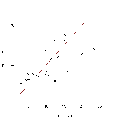
The mod.rh model does not appear to perform too bad after all. A few of the high observed values contribute greatly to the evaluation diagnostics. A couple of methods are available to assess the sensitivity of these results.
The first is to remove what could potentially be outliers from the data.
The second is to perform a sensitivity analysis which would include iterating the data sub-setting procedure and evaluate the models each time to get a sense how much the outcomes vary.
In the example below this is demonstrated by repeating the random subsetting 5 times. Note that you could do this many more times over.
Note also the removal of the set.seed function as we need to take a new subset for each iteration. This will also mean that the final
results shown below and what you generate will be slightly different.
# repeated random subsetting place to store results
validation.outs <- matrix(NA, nrow = 5, ncol = 6)

# repeat subsetting and model fitting
for (i in 1:5) {
  training <- sample(nrow(mod.data), 0.7 * nrow(mod.data), replace = FALSE)
  mod.rh <- lm(CEC ~ clay, data = mod.data[training, ], y = TRUE, x = TRUE)
  mod.rh.V <- predict(mod.rh, mod.data[-training, ])
  validation.outs[i, 1] <- i
  validation.outs[i, 2:6] <- as.matrix(goof(predicted = mod.rh.V, observed =   mod.data$CEC[-training]))}

validation.outs <- as.data.frame(validation.outs)
names(validation.outs) <- c("iteration", "R2", "concordance", "MSE", "RMSE", "bias")

# print outputs
validation.outs

##   iteration        R2 concordance       MSE     RMSE       bias
## 1         1 0.5582916   0.6735857 13.467984 3.669875  0.6320056
## 2         2 0.4282025   0.5200623 17.925045 4.233798 -1.1412116
## 3         3 0.6235765   0.7442635  5.734524 2.394687  0.2961916
## 4         4 0.4447690   0.5909275  9.697983 3.114159  0.2976717
## 5         5 0.3431210   0.4567065 21.587716 4.646258 -1.8841137
Even over just 5 repeats, the model evaluations bounce around a bit depending on the given calibration and out-of-bag data sets. As the data set being used here is relatively small, one might expect this type of sensitive behavior. It is also a good case in point to ensure if this type of cross-validation strategy is to be used, that it needs to be iterated/repeated over several times to ensure more robust predictions.
K-fold cross-validation
As the name suggests, k-fold cross-validation is about creating a defined number of folds or subsets in the whole data, fitting the model with a given number of folds and then evaluating the model with the other remaining folds. For example if we impose four folds in the available data, we could fit the model with three of the folds and validate on the fourth one. In the example below the folds are randomly assigned to each case, but could be imposed differently for example with a spatial clustering in order to implement a spatial cross-validation procedure.
In the example below we repeat the four fold cross-validation 1000 times, in which case we would call this a repeated four fold cross-validation.
# Set up matrix to store goodness of fit statistics for each model 4 fold
# repeated 1000 times = 4000 models
validation.outs <- matrix(NA, nrow = 4000, ncol = 6)

# repeat subsetting and model fitting
cnt <- 1
for (j in 1:1000) {
  # set up folds
  folds <- rep(1:4, length.out = nrow(mod.data))
  # random permutation
  rs <- sample(1:nrow(mod.data), replace = F)
  rs.folds <- folds[order(rs)]

  # model fitting for each combination of folds
  for (i in 1:4) {
    training <- which(rs.folds != i)
    mod.rh <- lm(CEC ~ clay, data = mod.data[training, ], y = TRUE, x = TRUE)
    mod.rh.V <- predict(mod.rh, mod.data[-training, ])
    validation.outs[cnt, 1] <- cnt
    validation.outs[cnt, 2:6] <- as.matrix(goof(predicted = mod.rh.V, observed = mod.data$CEC[-training]))
    cnt <- cnt + 1}}

# make the evaluation table a bit easier to decipher
validation.outs <- as.data.frame(validation.outs)
names(validation.outs) <- c("iteration", "R2", "concordance", "MSE", "RMSE", "bias")

# averaged goodness of fit measures
apply(validation.outs[, 2:6], 2, mean)

##           R2  concordance          MSE         RMSE         bias
##  0.442282110  0.572562985 14.530480367  3.744664092  0.006906522

# standard deviation of goodness of fit measures
apply(validation.outs[, 2:6], 2, sd)

##          R2 concordance         MSE        RMSE        bias
##  0.11891956  0.09799382  5.54250995  0.71281009  0.72051238
Bootstrapping
If the size of a data set has n number of cases, as described earlier, the bootstrap cross validation involves selecting n number of cases with replacement. However because sampling is done with replacement, only about 63% of cases are selected. The other 37% can therefore be used as an out-of-bag model evaluation dataset (Efron and Tibshirani 1997). Below we repeat the bootstrapping 4000 times and then estimate the averaged goodness of fit measures and the standard deviation of those too.
# Set up matrix to store goodness of fit statistics for each model of the 4000 models
validation.outs <- matrix(NA, nrow = 4000, ncol = 6)

# repeat subsetting and model fitting
for (j in 1:4000) {
  # sample with replacement
  rs <- sample(1:nrow(mod.data), replace = T)
  # get the unique cases
  urs <- unique(rs)
  # calibration data
  cal.dat <- mod.data[urs, ]
  # validation data
  val.dat <- mod.data[-urs, ]

  # model fitting
  mod.rh <- lm(CEC ~ clay, data = cal.dat, y = TRUE, x = TRUE)
  mod.rh.V <- predict(mod.rh, val.dat)
  validation.outs[j, 1] <- j
  validation.outs[j, 2:6] <- as.matrix(goof(predicted = mod.rh.V, observed = val.dat$CEC))}

validation.outs <- as.data.frame(validation.outs)
names(validation.outs) <- c("iteration", "R2", "concordance", "MSE", "RMSE", "bias")

# averaged goodness of fit meansures
apply(validation.outs[, 2:6], 2, mean)

##           R2  concordance          MSE         RMSE         bias
##  0.432680707  0.574861262 14.587025983  3.779626669  0.006002626

# standard deviation of goodness of fit meansures
apply(validation.outs[, 2:6], 2, sd)

##          R2 concordance         MSE        RMSE        bias
##  0.09327080  0.07662582  4.19643649  0.54911165  0.64825113
References
Brus, D., B. Kempen, and G.B.M. Heuvelink. 2011. “Sampling for Validation of Digital Soil Maps.” European Journal of Soil Science 62 (3): 394–407.
Efron, Bradley, and Robert Tibshirani. 1997. “Improvements on Cross-Validation: The .632+ Bootstrap Method.” Journal of the American Statistical Association 92 (438). [American Statistical Association, Taylor & Francis, Ltd.]: 548–60. http://www.jstor.org/stable/2965703.
Gruijter, J. de, D.J. Brus, M.F.P. Bierkens, and M. Knotters. 2006. Sampling for Natural Resource Monitoring. Berlin Heidelberg: Springer-Verlag.
Hastie, T., R. Tibshirani, and J Friedman. 2001. The Elements of Statistical Learning. New York, NY: Springer.
Lovelace, R., J Nowosad, and J Muenchow. 2019. Geocomputation with R. Chapman; Hall/CRC.