CODE:
Get the code used in the sections about preparatory and exploratory data analysis
Soil depth functions
Skip to fitting splines to multiple soil profiles
The traditional method of sampling soil involves dividing a soil profile into horizons. The number of horizons and the position of each are generally based on attributes easily observed in the field, such as morphological soil properties (Bishop et al. 1999). From each horizon, a bulk sample is taken and it is assumed to represent the average value for a soil attribute over the depth interval from which it is sampled.
There are some issues with this approach, particularly from a pedological perspective and secondly from the difficulty in using this legacy data within a Digital Soil Mapping (DSM) framework where we wish to know the continuous variability of a soil both in the lateral and vertical dimensions. From the pedological perspective soil generally varies continuously with depth; however, representing the soil attribute value as the average over the depth interval of horizons leads to discontinuous or stepped profile representations.
Difficulties can arise in situations where one wants to know the value of an attribute at a specified depth. The second issue is regarding DSM and is where we use a database of soil profiles to generate a model of soil variability in the area in which they exist. Because observations at each horizon for each profile will rarely be the same between any two profiles, it then becomes difficult to build a model where predictions are made at a set depth or at standardized depth intervals.
Exceptions to this include so-called one-step models such as those described in Orton et al. (2016) and Poggio and Gimona (2014), but to date have not been widely used despite their reported advantages (in terms of predictive skill and efficiency) over the approach described below and then in subsequent pages which has been described as a two-step approach.
Legacy soil data is too valuable to do away with, and thus needs to be shaped to suit the purposes of the map producer, such that one needs to be able to derive a continuous function using the available horizon data as some input.
This can be done with many methods including polynomials and exponential decay type depth functions. A more general continuous depth function is the equal-area quadratic spline function. The usage and mathematical expression of this function have been detailed in Ponce-Hernandez et al. (1986), Bishop et al. (1999), and Malone et al. (2009).
A useful feature of the spline function is that it is mass preserving (hence the name equal area), or in other words the original data is preserved and can be retrieved again via integration of the continuous spline.
Compared to exponential decay functions where the goal is in defining the actual parameters of the decay function, the spline parameters are the values of the soil attribute at the standard depths that are specified by the user. This is a useful feature, because firstly, one can harmonize a whole collection of soil profile data and then explicitly model the soil for a specified depth. For example the GlobalSoilMap.net project (Arrouays et al. 2014) has a specification that digital soil maps be created for each target soil variable for the 0-5cm, 5-15cm, 15-30cm, 30-60cm, 60-100cm, and 100-200cm depth intervals. In this case, the mass-preserving splines can be fitted to the observed data, then values can be extracted from them at the required depths, and are then ready for exploratory analysis and spatial modelling.
In the following, we will use legacy soil data and the spline function to prepare data to be used in a DSM framework. This will specifically entail fitting splines to all the available soil profiles and then through a process of harmonization, integrate the splines to generate harmonized depths of each observation.
Fit mass preserving splines with R
Skip to fitting splines to multiple soil profiles
The following demonstrates mass-preserving spline fitting using a single soil profile example for which there are measurements of soil carbon density to a given maximum depth.
We can fit a spline to the maximum soil depth, or alternatively any depth that does not exceed the maximum soil depth. The function used for fitting splines is called ea_spline and is from the ithir package.
Look at the help file for further information on this function. For example, there is further information about how the ea_spline function can also accept data of class SoilProfileCollection from the aqp package in addition to data of the generic data.frame class.
In the example below the input data is of class data.frame. The data we need, oneProfile is in the ithir package. Lets also load a few of the other important R packages that will be encountered in this section too.
#Load ithir library
library(ithir)

#ithir dataset
data(oneProfile)
str(oneProfile)

## 'data.frame':    8 obs. of  4 variables:
##  $ Soil.ID       : int  1 1 1 1 1 1 1 1
##  $ Upper.Boundary: int  0 10 30 50 70 120 250 350
##  $ Lower.Boundary: int  10 20 40 60 80 130 260 360
##  $ C.kg.m3.      : num  20.72 11.71 8.23 6.3 2.4 ...
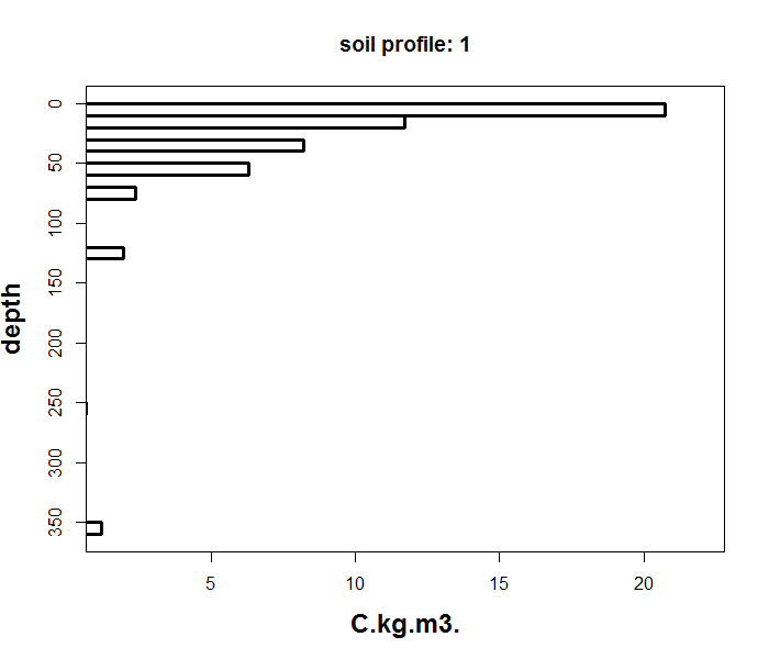
As you can see above, the data table shows the soil depth information and carbon density values for a single soil profile. Note the discontinuity of the observed depth intervals which can also be observed in the figure below.
The ea_spline function will predict a continuous function from the top of the soil profile to the maximum soil depth, such that it will interpolate values both within the observed depths and between the depths where there is no observation.
To parametize the ea_spline function, we could accept the defaults, however it might be suitable to change the lam and d parameters to suit the objective of the analysis being undertaken. lam is the lambda parameter which controls the smoothness or fidelity of the spline. Increasing this value will make the spline more rigid. Decreasing it towards zero will make the spline more flexible such that it will follow near directly the observed data.
A sensitivity analysis is generally recommended in order to optimize this parameter. From experience a lam value of 0.1 works well generally for most soil properties, and is the default value for the function.
The d parameter represents the depth intervals at which we want to get soil values for. This is a harmonization process where regardless of which depths soil was observed at, we can derive the soil values for regularized and standard depths.
In practice, the continuous spline function is first fitted to the data, then we get the integrals of this function to determine the values of the soil at the standard depths. d is a matrix, but on the basis of the default values, what it is indicating is that we want the values of soil at the following depth
intervals: 0-5cm, 5-15cm, 15-30cm, 30-60cm, 60-100cm, and 100-200cm.
These depths are specified depths determined for the GlobalSoilMap.net project (Arrouays et al. 2014). Naturally, one can alter these values to suit there own particular requirements. To fit a spline to the carbon density values of the oneProfile data, the following script could be used:
eaFit <- ithir::ea_spline(oneProfile, var.name="C.kg.m3.",
        d= t(c(0,5,15,30,60,100,200)),lam = 0.1, vlow=0,
        show.progress=FALSE )
str(eaFit)

## List of 4
##  $ harmonised    :'data.frame':  1 obs. of  8 variables:
##   ..$ id        : num 1
##   ..$ 0-5 cm    : num 21.1
##   ..$ 5-15 cm   : num 15.8
##   ..$ 15-30 cm  : num 9.91
##   ..$ 30-60 cm  : num 7.2
##   ..$ 60-100 cm : num 2.75
##   ..$ 100-200 cm: num 1.72
##   ..$ soil depth: num 360
##  $ obs.preds     :'data.frame':  8 obs. of  6 variables:
##   ..$ Soil.ID       : num [1:8] 1 1 1 1 1 1 1 1
##   ..$ Upper.Boundary: num [1:8] 0 10 30 50 70 120 250 350
##   ..$ Lower.Boundary: num [1:8] 10 20 40 60 80 130 260 360
##   ..$ C.kg.m3.      : num [1:8] 20.72 11.71 8.23 6.3 2.4 ...
##   ..$ predicted     : num [1:8] 19.86 12.46 8.27 6.2 2.56 ...
##   ..$ FID           : num [1:8] 1 1 1 1 1 1 1 1
##  $ splineFitError:'data.frame':  1 obs. of  2 variables:
##   ..$ rmse   : num 0.41
##   ..$ rmseiqr: num 0.0561
##  $ var.1cm       : num [1:200, 1] 21.6 21.4 21.2 20.8 20.3 ...
The output of the function is a list, where the first element is a data.frame (harmonized) which are the predicted spline estimates at the specified depth intervals. The second element (obs.preds) is another data.frame but contains the observed soil data together with spline predictions for the actual depths of observation for each soil profile. The third element (splineFitError) is a data.frame that stores the profile root mean square error (RMSE) estimate and the normalized root-mean-square (nRMSE) deviation. The interquartile range
is used as the denominator in the nRMSE. This value is an estimate of
the magnitude of difference between observed values and associated
predicted values with each profile. The fourth element, (var.1cm) is a
matrix which stores the spline predictions of the depth function at (in
this case) 1cm resolution. Each column represents a given soil profile
and each row represents an incremental 1cm depth increment to the
maximum depth we wish to extract values for, or to the maximum observed
soil depth (which ever is smallest).
It is often more amenable to visualize the performance of the spline
fitting. Subsequently, plotting the outputs of ea_spline is made
possible by the associated plot_ea_spline function (see help file for
use of this function):
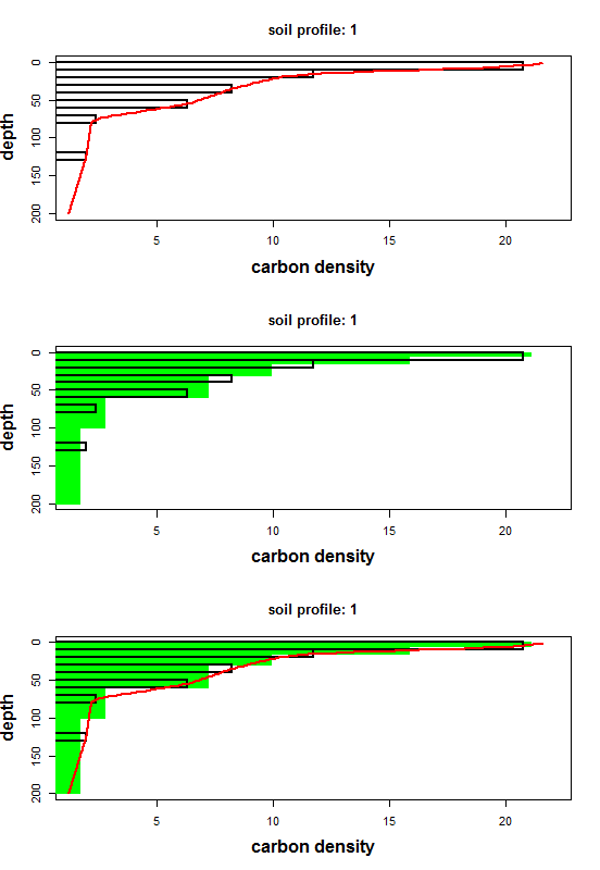
par(mfrow=c(3,1))
for (i in 1:3){
  ithir::plot_ea_spline(splineOuts=eaFit,
  d= t(c(0,5,15,30,60,100,200)), maxd=200,
  type=i, plot.which=1, label="carbon density")}
The plot_ea_spline function is a basic function without too much
control over the plotting parameters, except there are three possible
themes of plot output that one can select. This is controlled by the
type parameter. Type = 1 is to return the observed soil data plus
the continuous spline (default). Type = 2 is to return the observed
data plus the averages of the spline at the specified depth intervals.
Type = 3 is to return the observed data, spline averages and
continuous spline. The script above results in producing all three
possible plots, and is shown on the figure below.
Fitting spline to multiple soil profiles.
The above example is just a demonstration of the ea_spline function
with the very unlikely scenario of a single soil profile. A normal use
case is to fit splines for a collection of soil profiles.
The implementation is exactly the same.
All the work happens within the function in terms of processing sequentially each given profile. The input data is also the same, but you need to be mindful that each profile is given a unique identifier so that the processing goes without a hitch. This unique profile can either be numerical or character type or a combination of both.
The data for this example is called Carbon_10sites.
Download the file and it is called Carbon_10sites.csv. It is 10 soil
profiles with measured soil carbon stocks.
Note that the ea_spline function is very fast despite no re-factoring improvements. This is because the internal computations are relatively simple with no overheads or other package dependencies. The size of the profiles to
process is basically the only impediment to time, but experience has
demonstrated that the current function can process tens of thousands in
soil profiles in a few minutes.
# load data
Carbon_10sites<- read.csv("~/Carbon_10sites.csv")

# fit spline to each profile
eaFit <- ithir::ea_spline(obj = Carbon_10sites,
var.name="C.kg.m3.", d= t(c(0,5,15,30,60,100,200)),lam = 0.1, vlow=0, show.progress=FALSE )

str(eaFit)

## List of 4
##  $ harmonised    :'data.frame':  10 obs. of  8 variables:
##   ..$ id        : num [1:10] 1 2 3 4 5 6 7 8 9 10
##   ..$ 0-5 cm    : num [1:10] 28.78 23.68 12.45 7.69 7.51 ...
##   ..$ 5-15 cm   : num [1:10] 18.62 14.67 9.3 6.35 6.94 ...
##   ..$ 15-30 cm  : num [1:10] 10.47 6.48 6.6 5.49 6.47 ...
##   ..$ 30-60 cm  : num [1:10] 9.22 6.65 5.59 5.58 6 ...
##   ..$ 60-100 cm : num [1:10] 5.31 6.13 3.99 4.08 4.41 ...
##   ..$ 100-200 cm: num [1:10] 3.13 3.31 1.18 1.85 2.72 ...
##   ..$ soil depth: num [1:10] 260 260 260 260 260 259 260 260 253 260
##  $ obs.preds     :'data.frame':  62 obs. of  6 variables:
##   ..$ Level.Soil.ID : num [1:62] 1 1 1 1 1 1 2 2 2 2 ...
##   ..$ Upper.Boundary: num [1:62] 0 10 30 70 120 250 0 10 30 70 ...
##   ..$ Lower.Boundary: num [1:62] 8 20 40 80 130 260 10 20 40 80 ...
##   ..$ C.kg.m3.      : num [1:62] 28.69 11.94 10.59 5.28 3.76 ...
##   ..$ predicted     : num [1:62] 27.6 13.06 10.48 5.35 3.77 ...
##   ..$ FID           : num [1:62] 1 1 1 1 1 1 2 2 2 2 ...
##  $ splineFitError:'data.frame':  10 obs. of  2 variables:
##   ..$ rmse   : num [1:10] 0.642 0.6536 0.1653 0.1098 0.0462 ...
##   ..$ rmseiqr: num [1:10] 0.0861 0.2069 0.0321 0.0343 0.0149 ...
##  $ var.1cm       : num [1:200, 1:10] 29.9 29.6 29 28.2 27.2 ...
Now with more than one soil profile, it is perhaps easier to make sense
of the function outputs, in particular the eaFit$harmonised element
which stores on each line the fitted values at the specified soil
depths. The soil.depth column is also helpful too in helping interpret
the fitted outputs.
References
Arrouays, D, N McKenzie, J Hempel, A Richer de Forges, and A McBratney, eds. 2014. GlobalSoilMap: Basis of the Global Spatial Soil Information System. CRC Press.
Bishop, T F A, A B McBratney, and G M Laslett. 1999. “Modelling Soil Attribute Depth Functions with Equal-Area Quadratic Smoothing Splines.” Geoderma 91: 27–45.
Malone, B P, A B McBratney, B Minasny, and G M Laslett. 2009. “Mapping Continuous Depth Functions of Soil Carbon Storage and Available Water Capacity.” Geoderma 154: 138–52.
Orton, T. G., M. J. Pringle, and T. F. A. Bishop. 2016. “A One-Step Approach for Modelling and Mapping Soil Properties Based on Profile Data Sampled over Varying Depth Intervals.” Geoderma 262: 174–86. http://www.sciencedirect.com/science/article/pii/S0016706115300422.
Poggio, Laura, and Alessandro Gimona. 2014. “National Scale 3D Modelling of Soil Organic Carbon Stocks with Uncertainty Propagation – an Example from Scotland.” Geoderma 232-234: 284–99. http://www.sciencedirect.com/science/article/pii/S0016706114002006.
Ponce-Hernandez, R, F H C Marriott, and P H T Beckett. 1986. “An Improved Method for Reconstructing a Soil Profile from Analysis of a Small Number of Samples.” Journal of Soil Science 37: 455–67.