Introduction
Advances in computing and information technologies have ushered in the age of big data and powerful tools across all fields — including environmental and spatial sciences. These developments have sparked global efforts to build spatial data infrastructures that support the collection, management, and use of spatial information.
Soil science contributes to this through the development of regional, continental, and global soil databases. Some of these are now operational and used in applications such as land resource assessment and risk evaluation (Lagacherie & McBratney, 2006).
However, these databases are often incomplete and insufficiently detailed. Most rely on digitised conventional soil surveys, which are expensive, slow to produce, and increasingly rare due to reduced funding since the 1980s (Hartemink & McBratney, 2008). As a result, large gaps remain in the spatial coverage and quality of available soil data.
To overcome this, spatial soil information systems need to evolve — from storing only digitised legacy maps to producing new soil maps ab initio. This is the central aim of Digital Soil Mapping (DSM).
Digital Soil Mapping (DSM) is the creation and population of spatial soil information systems using numerical models that infer the spatial and temporal variation of soil types and properties from soil observations and related environmental variables.
The scorpan Model
The concepts and methodologies for DSM were formalised by McBratney, Mendonça Santos, and Minasny (2003). They introduced the scorpan approach — a framework for predicting soil attributes based on environmental variables. This was influenced by earlier works by Jenny (1941) and Dokuchaev.
scorpan is a mnemonic for the environmental factors influencing soil:
- s: soil (existing properties)
- c: climate
- o: organisms (vegetation, fauna)
- r: relief (topography)
- p: parent material
- a: age
- n: spatial location
The model is expressed as:
S = f(s, c, o, r, p, a, n) + ϵ
or more generally: S = f(Q) + ϵ
Where S is the soil property or class at a location, f(Q) is a deterministic model using the scorpan factors, and ϵ is the spatially dependent residual (unexplained variation).
This formulation is known as scorpan-kriging, where the deterministic model f(Q) is complemented by kriging of residuals to capture spatial dependence.
Covariates used in f(Q) may include:
- Digital elevation models (e.g. slope, aspect, MRVBF)
- Remote sensing (e.g. Landsat, radiometrics)
- Geological and soil survey maps
- Legacy soil profile data
Residuals (ϵ) are modelled via geostatistical methods (e.g. variograms and kriging), assuming spatial structure exists due to unmeasured interactions or model limitations.
What if No Point Data Exists?
The scorpan-kriging approach requires point observations. But what if they’re not available?
Minasny & McBratney (2010) proposed a decision tree to guide DSM based on available legacy data. This framework also applies beyond global mapping — it’s useful at any scale.
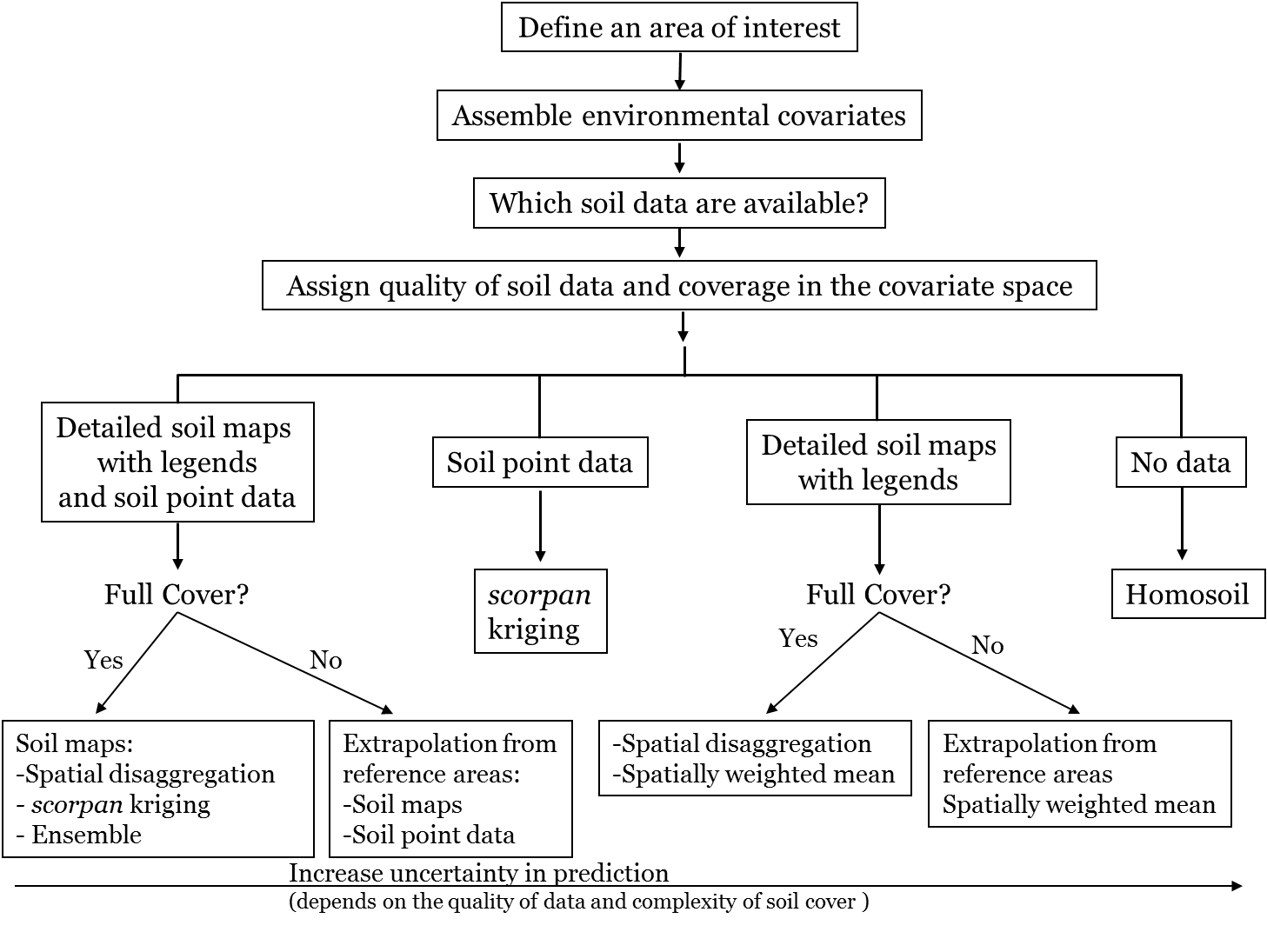
Mapping Scenarios Based on Available Data
1. Point data only
→ Use scorpan-kriging.
2. Soil maps and point data
→ Combine approaches (e.g. Malone et al., 2014).
3. Only soil maps
→ Estimate soil properties using mapping unit information, such as modal profile data.
Approaches include spatially weighted means based on map unit composition (e.g. Odgers, Libohova & Thompson, 2012).
4. Disaggregation of complex map units
→ Apply algorithms like DSMART (Odgers et al., 2014) to decompose and assign probabilities to soil classes.
→ Use PROPR (Odgers, McBratney & Minasny, 2015) to convert class probabilities and modal profiles into soil property estimates.
5. No data at all
→ Use analogue approaches based on soil homology between a reference area and a target region.
See Malone, Jha & Minasny (2016) for examples of extrapolating from similar environments.
Purpose of This Course
This course focuses on practical DSM implementation, with particular emphasis on scorpan-kriging and disaggregation of polygonal soil maps. The goal is to help you:
- Apply DSM theory using
R - Work with both continuous and categorical soil data
- Understand soil covariates and preprocessing
- Produce, evaluate, and update digital soil maps
- Explore digital soil assessment for land use and suitability
- Understand uncertainty and validation in DSM
- Learn about analogues like Homosoil for data-sparse regions
The course is hands-on — with a “how-to” spirit — and leans heavily on worked examples using R. It also explores operational applications such as validation of soil maps and decision-support tools like digital soil assessment (DSA) (Carré et al., 2007).
References
Bui, E.N., and C. J. Moran. 2003. “A Strategy to Fill Gaps in Soil Survey over Large Spatial Extents: An Example from the Murray-Darling Basin of Australia.” Geoderma 111: 21–41.
Carre, F., Alex B. McBratney, Thomas Mayr, and Luca Montanarella. 2007. “Digital Soil Assessments: Beyond Dsm.” Geoderma 142 (1-2): 69–79. https://doi.org/http://dx.doi.org/10.1016/j.geoderma.2007.08.015.
Hartemink, A E, and A B McBratney. 2008. “A Soil Science Renaissance.” Geoderma 148: 123–29.
Jenny, H. 1941. Factors of Soil Formation. New York: McGraw-Hill.
Lagacherie, P, and A B McBratney. 2006. “Digital Soil Mapping: An Introductory Perspective.” In, edited by P Lagacherie, A B McBratney, and M Voltz, 3–22. Amsterdam: Elsevier.
Malone, B P, S K Jha, and A B Minasny B McBratney. 2016. “Comparing Regression-Based Digital Soil Mapping and Multiple-Point Geostatistics for the Spatial Extrapolation of Soil Data.” Geoderma 262: 243–53.
Malone, B P, B Minasny, N P Odgers, and A B McBratney. 2014. “Using Model Averaging to Combine Soil Property Rasters from Legacy Soil Maps and from Point Data.” Geoderma 232-234: 34–44.
McBratney, A B, M L Mendonca Santos, and B Minasny. 2003. “On Digital Soil Mapping.” Geoderma 117: 3–52.
Minasny, B, and A B McBratney. 2010. “Digital Soil Mapping: Bridging Research, Environmental Application, and Operation.” In, edited by J L Boettinger, D W Howell, A C Moore, A E Hartemink, and Kienast-Brown S, 429–25. Dordrecht: Springer.
Odgers, N P, Z Libohova, and J A Thompson. 2012. “Equal-Area Spline Functions Applied to a Legacy Soil Database to Create Weighted-Means Maps of Soil Organic Carbon at a Continental Scale.” Georderma 189-190: 153–63.
Odgers, N P, A B McBratney, and B Minasny. 2015. “Digital Soil Property Mapping and Uncertainty Estimation Using Soil Class Probability Rasters.” Geoderma 237-238: 190–98.
Odgers, N P, W Sun, A B McBratney, B Minasny, and D Clifford. 2014. “Disaggregating and Harmonising Soil Map Units Through Resampled Classification Trees.” Geoderma 214-215: 91–100.