CODE:
Get the code used for this section here
Linear models: the basics
The lm function, model formulas, and statistical output
In R several classical statistical models can be implemented using one
function: lm (for linear model). The lm function can be used for
simple and multiple linear regression, analysis of variance (ANVOVA),
and analysis of covariance (ANCOVA). The help file for lm lists the
following.
lm(formula, data, subset, weights, na.action, method = ``qr'', model = TRUE, x = FALSE, y = FALSE, qr = TRUE, singular.ok = TRUE, contrasts = NULL, offset, ...)
The first argument in the lm function call (formula) is where you
specify the structure of the statistical model. This approach is used in
other R functions as well, such as glm, gam, and others, which we
will later investigate. The most common structures of a statistical
model are:
y ∼ x :Simple linear regression of y on x
y ∼ x + z :Multiple regression of y on x and z
There are many others, but it is these model structures that are used in one form or another for digital soil mapping.
There is some similarity between the statistical output in R and in
other statistical software programs. However, by default, R usually
gives only basic output. More detailed output can be retrieved with the
summary function. For specific statistics, you can use extractor
functions, such as coef or deviance. Output from the lm function
is of the class lm, and both default output and specialized output
from extractor functions can be assigned to objects (this is of course
true for other model objects as well). This quality is very handy when
writing code that uses the results of statistical models in further
calculations or in compiling summaries.
Linear regression
To demonstrate simple linear regression in R, we will again use the
soil.data set. Here we will regress CEC content on clay.
    library(ithir)
    data(USYD_soil1)
    soil.data <- USYD_soil1
    summary(cbind(clay = soil.data$clay, CEC = soil.data$CEC))

    ##       clay            CEC
    ##  Min.   : 5.00   Min.   : 1.900
    ##  1st Qu.:15.00   1st Qu.: 5.350
    ##  Median :21.00   Median : 8.600
    ##  Mean   :26.95   Mean   : 9.515
    ##  3rd Qu.:37.00   3rd Qu.:12.110
    ##  Max.   :68.00   Max.   :28.210
    ##  NA's   :17      NA's   :5
The (alternative) hypothesis here is that clay content is a good predictor of CEC. As a start, let us have a look at what the data looks like.
plot(soil.data$clay, soil.data$CEC)
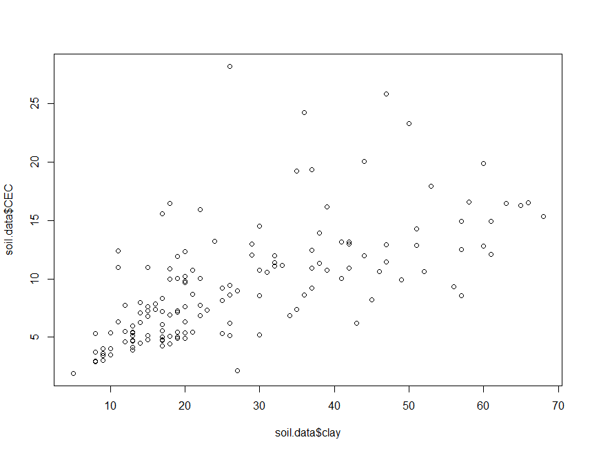
There appears to be some meaningful relationship. To fit a linear model,
we can use the lm function:
    mod.1 <- lm(CEC ~ clay, data = soil.data, y = TRUE, x = TRUE)
    mod.1

    ##
    ## Call:
    ## lm(formula = CEC ~ clay, data = soil.data, x = TRUE, y = TRUE)
    ##
    ## Coefficients:
    ## (Intercept)         clay
    ##      3.7791       0.2053
R returns only the call and coefficients by default. You can get more
information using the summary function.
    summary(mod.1)

    ##
    ## Call:
    ## lm(formula = CEC ~ clay, data = soil.data, x = TRUE, y = TRUE)
    ##
    ## Residuals:
    ##     Min      1Q  Median      3Q     Max
    ## -7.1829 -2.3369 -0.6767  1.0185 19.0924
    ##
    ## Coefficients:
    ##             Estimate Std. Error t value Pr(>|t|)
    ## (Intercept)  3.77913    0.63060   5.993 1.58e-08 ***
    ## clay         0.20533    0.02005  10.240  < 2e-16 ***
    ## ---
    ## Signif. codes:  0 '***' 0.001 '**' 0.01 '*' 0.05 '.' 0.1 ' ' 1
    ##
    ## Residual standard error: 3.783 on 144 degrees of freedom
    ##   (20 observations deleted due to missingness)
    ## Multiple R-squared:  0.4214, Adjusted R-squared:  0.4174
    ## F-statistic: 104.9 on 1 and 144 DF,  p-value: < 2.2e-16
Clay does appear to be a significant predictor of CEC as one would
generally surmise when applying our soil science knowledge. As mentioned
above, the output from the lm function is an object of class lm.
These objects are lists that contain at least the following elements
(you can find this list in the help file for lm):
coefficients: a named vector of model coefficientsresiduals: model residuals (observed - predicted values)fitted.value: the fitted mean valuesrank: a numeric rank of the fitted linear modelweights: (only for weighted fits) the specified weightsdf.residual: the residual degrees of freedomcall: the matched callterms: the terms object usedcontrasts: (only where relevant) the contrasts usedxlevels: (only where relevant) a record of the levels of the factors used in fittingoffset: the offset used (missing if none were used)y: if requested, the response usedx: if requested, the model matrix usedmodel: if requested (the default), the model frame usedna.action: (where relevant) information returned by model frame on the handling ofNAs
To get at the elements listed above, you can simply index the lm
object, i.e. call up part of the list.
    mod.1$coefficients

    ## (Intercept)        clay
    ##   3.7791256   0.2053256
However, R has several extractor functions designed precisely for
pulling data out of statistical model output. Some of the most commonly
used ones are: add1, alias, anova, coef, deviance, drop1,
effects, family, formula, kappa, labels, plot, predict,
print, proj, residuals, step, summary, and vcov. For
example:
    coef(mod.1)

    ## (Intercept)        clay
    ##   3.7791256   0.2053256

    head(residuals(mod.1))

    ##          1          2          3          4          6          7
    ## -0.1317300 -1.7217300 -2.5617300 -2.5017300 -0.5226822 -2.0370556
As mentioned before, the summary function is a generic function. What
it does and what it returns is dependent on the class of its first
argument. Here is a list of what is available from the summary
function for this model:
    names(summary(mod.1))

    ##  [1] "call"          "terms"         "residuals"     "coefficients"
    ##  [5] "aliased"       "sigma"         "df"            "r.squared"
    ##  [9] "adj.r.squared" "fstatistic"    "cov.unscaled"  "na.action"
To extract some of the information in the summary which is of a list
structure, we would use:
    summary(mod.1)[[4]]

    ##              Estimate Std. Error   t value     Pr(>|t|)
    ## (Intercept) 3.7791256 0.63060292  5.992877 1.577664e-08
    ## clay        0.2053256 0.02005048 10.240431 7.910414e-19
To look at the statistical summary. What is the R2 of
mod.1? Answer:
    summary(mod.1)[["r.squared"]]

    ## [1] 0.4213764
This flexibility is useful, but makes for some redundancy in R. For
many model statistics, there are three ways to get your data: an
extractor function (such as coef), indexing the lm object, and
indexing the summary function. The best approach is to use an
extractor function whenever you can. In some cases, the summary
function will return results that you can not get by indexing or using
extractor functions.
Once we have fit a model in R, we can generate predicted values using
the predict function.
    head(predict(mod.1))

    ##         1         2         3         4         6         7
    ##  5.421730  5.421730  5.421730  5.421730 15.482682  5.627056
Lets plot the observed vs. the predict from this model.
plot(mod.1$y, mod.1$fitted.values)
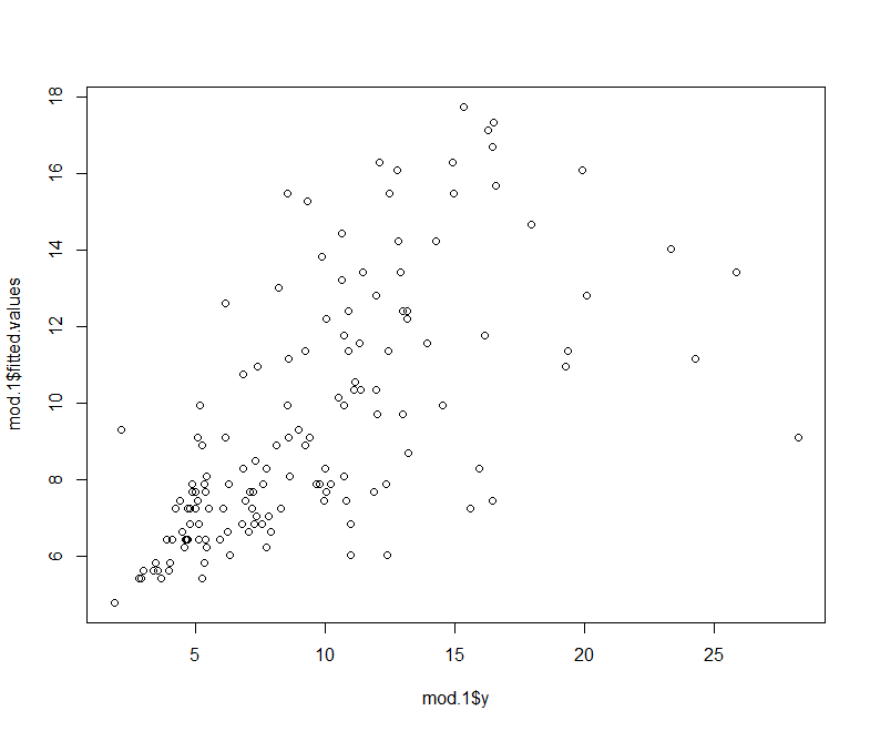
As we will see later on, the predict function works for a whole range
of statistical models in R. Not just lm objects. We can treat the
predictions as we would any vector. For example we can add them to the
above plot or put them back in the original data frame. The predict
function can also give confidence and prediction intervals.
    head(predict(mod.1, int = "conf"))

    ##         fit       lwr       upr
    ## 1  5.421730  4.437845  6.405615
    ## 2  5.421730  4.437845  6.405615
    ## 3  5.421730  4.437845  6.405615
    ## 4  5.421730  4.437845  6.405615
    ## 6 15.482682 14.152940 16.812425
    ## 7  5.627056  4.673657  6.580454
A quick way to demonstrate multiple linear regression in R, we will
regress CEC on clay plus the exchangeable cations: ExchNa and
ExchCa. First lets subset these data out, then get their summary
statistics.
    subs.soil.data <- soil.data[, c("clay", "CEC", "ExchNa", "ExchCa")]
    summary(subs.soil.data)

    ##       clay            CEC             ExchNa           ExchCa
    ##  Min.   : 5.00   Min.   : 1.900   Min.   :0.0000   Min.   : 1.010
    ##  1st Qu.:15.00   1st Qu.: 5.350   1st Qu.:0.0200   1st Qu.: 2.920
    ##  Median :21.00   Median : 8.600   Median :0.0500   Median : 4.610
    ##  Mean   :26.95   Mean   : 9.515   Mean   :0.2563   Mean   : 5.353
    ##  3rd Qu.:37.00   3rd Qu.:12.110   3rd Qu.:0.1500   3rd Qu.: 7.240
    ##  Max.   :68.00   Max.   :28.210   Max.   :6.8100   Max.   :25.390
    ##  NA's   :17      NA's   :5        NA's   :5        NA's   :5
A quick way to look for relationships between variables in a data frame
is with the cor function. Note the use of the na.omit function.
    cor(na.omit(subs.soil.data))

    ##             clay       CEC      ExchNa      ExchCa
    ## clay   1.0000000 0.6491351  0.17104962  0.54615778
    ## CEC    0.6491351 1.0000000  0.33369789  0.87570029
    ## ExchNa 0.1710496 0.3336979  1.00000000 -0.02055496
    ## ExchCa 0.5461578 0.8757003 -0.02055496  1.00000000
To visualize these relationships, we can use pairs.
pairs(na.omit(subs.soil.data))
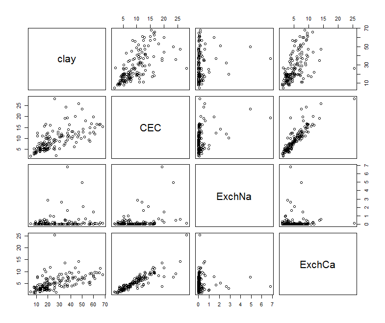
There are some interesting relationships here. Now for fitting the model:
    mod.2 <- lm(CEC ~ clay + ExchNa + ExchCa, data = subs.soil.data)
    summary(mod.2)

    ##
    ## Call:
    ## lm(formula = CEC ~ clay + ExchNa + ExchCa, data = subs.soil.data)
    ##
    ## Residuals:
    ##     Min      1Q  Median      3Q     Max
    ## -5.2008 -0.7065 -0.0470  0.6455  9.4025
    ##
    ## Coefficients:
    ##             Estimate Std. Error t value Pr(>|t|)
    ## (Intercept) 1.048318   0.274264   3.822 0.000197 ***
    ## clay        0.050503   0.009867   5.119 9.83e-07 ***
    ## ExchNa      2.018149   0.163436  12.348  < 2e-16 ***
    ## ExchCa      1.214156   0.046940  25.866  < 2e-16 ***
    ## ---
    ## Signif. codes:  0 '***' 0.001 '**' 0.01 '*' 0.05 '.' 0.1 ' ' 1
    ##
    ## Residual standard error: 1.522 on 142 degrees of freedom
    ##   (20 observations deleted due to missingness)
    ## Multiple R-squared:  0.9076, Adjusted R-squared:  0.9057
    ## F-statistic: 465.1 on 3 and 142 DF,  p-value: < 2.2e-16
For much of the remainder of the exercises, we will be investigating
these regression type relationships using a variety of different model
types for soil spatial prediction. These fundamental modelling concepts
of the lm will become useful as we progress ahead.
Exercises
-
Using the
soil.dataset firstly generate a correlation matrix of all the soil variables. -
Choose two variables that you think would be good to regress against each other, and fit a model. Is the model any good? Can you plot the observed vs. predicted values? Can you draw a line of concordance (maybe want to consult an appropriate help file to do this). Something a bit trickier: Can you add the predictions to the data frame
soil.datacorrectly. -
Now repeat what you did for the previous question, except this time perform a multiple linear regression i.e. use more than 1 predictor variable to make a prediction of the variable you are targeting.