CODE:
Get the code used for this section here
Logical thinking and algorithm development
One of the advantages of using a scripting language such as R is that
we can develop algorithms or script a set of commands for
problem-solving. We illustrate this by developing an algorithm for
generating a catena, or more correctly, a digital toposequence from a
digital elevation model (DEM). To make it more interesting, we will not
use any function from external libraries other than basic R functions.
Before scripting, it is best to write out the algorithm or sequence of
routines to use.
A toposequence can be described as a transect (not necessarily a straight line) which begins at a hilltop and ends at a valley bottom or a stream (Odgers, McBratney, and Minasny 2008). To generate a principal toposequence, one can start from the highest point in an area. If we numerically consider a rainfall as a discrete packet of precipitation that falls on the highest elevation pixel, then this precipitation will mostly move to its neighbor with the highest slope. As a DEM is stored in matrix format, we simply look around its 3 x 3 neighbors and determine which pixel is the lowest elevation. The algorithm for principal toposequence can be written as:
- Determine the highest point in an area.
- Determine its 3 x 3 neighbor, and determine whether there are lower points?
- If yes, set the lowest point as the next point in the toposequence, and then repeat step 2. If no, the toposequence has ended.
To facilitate the 3 x 3 neighbor search in R, we can code the
neighbors using its relative coordinates. If the current cell is
designated as [0,0], then its left neighbor is [−1,0], and so
on. We can visualize it as follows in the below figure.

If we designate the current cell [0,0] as z1, the function below
will look for the lowest neighbor for pixel z1 in a DEM.
    # function to find the lowest 3 x 3 neighbor
    find_steepest <- function(dem, row_z, col_z) {
        z1 = dem[row_z, col_z]  #elevation
        # return the elevation of the neighboring values
        dir = c(-1, 0, 1)  #neighborhood index
        nr = nrow(dem)
        nc = ncol(dem)
        pz = matrix(data = NA, nrow = 3, ncol = 3)  #placeholder for the values
        for (i in 1:3) {
            for (j in 1:3) {
                if (i != 0 & j != 0) {
                    ro <- row_z + dir[i]
                    co <- col_z + dir[j]
                    if (ro > 0 & co > 0 & ro < nr & co < nc) {
                      pz[i, j] = dem[ro, co]
                    }
                }
            }
        }

        pz <- pz - z1  # difference of neighbors from centre value
        # find lowest value
        min_pz <- which(pz == min(pz, na.rm = TRUE), arr.ind = TRUE)
        row_min <- row_z + dir[min_pz[1]]
        col_min <- col_z + dir[min_pz[2]]
        retval <- c(row_min, col_min, min(pz, na.rm = TRUE))
        return(retval)  #return the minimum
    }
The principal toposequence code can be implemented as follows. First we
load in a small dataset called topo_dem from the ithir package.
    library(ithir)
    data(topo_dem)
    str(topo_dem)

    ##  num [1:109, 1:110] 121 121 120 118 116 ...
    ##  - attr(*, "dimnames")=List of 2
    ##   ..$ : NULL
    ##   ..$ : chr [1:110] "V1" "V2" "V3" "V4" ...
Now we want to create a data matrix to store the result of the
toposequence i.e. the row, column, and elevation values that are
selected using the find_steepest function.
transect <- matrix(data = NA, nrow = 20, ncol = 3)
Now we want to find within that matrix that maximum elevation value and its corresponding row and column position.
    max_elev <- which(topo_dem == max(topo_dem), arr.ind = TRUE)
    row_z = max_elev[1]  # row of max_elev
    col_z = max_elev[2]  # col of max_elev
    z1 = topo_dem[row_z, col_z]  # max elevation

    # Put values into the first entry of the transect object
    t <- 1
    transect[t, 1] = row_z
    transect[t, 2] = col_z
    transect[t, 3] = z1
    lowest = FALSE
Below we use the find_steepest function. It is embedded into a while
conditional loop, such that the routine will run until neither of the
surrounding neighbors are less than the middle pixel or z1. We use the
break function to stop the routine when this occurs. Essentially, upon
each iteration, we use the selected z1 to find the lowest value pixel
from it, which in turn becomes the next selected z1 and so on until
the values of the neighborhood are no longer smaller than the selected
z1.
    # iterate down the hill until lowest point
    while (lowest == FALSE) {
        result <- find_steepest(dem = topo_dem, row_z, col_z)  # find steepest neighbor
        t <- t + 1
        row_z = result[1]
        col_z = result[2]
        z1 = topo_dem[row_z, col_z]
        transect[t, 1] = row_z
        transect[t, 2] = col_z
        transect[t, 3] = z1
        if (result[3] >= 0)
            {
                lowest == TRUE
                break
            }  # if found lowest point
    }
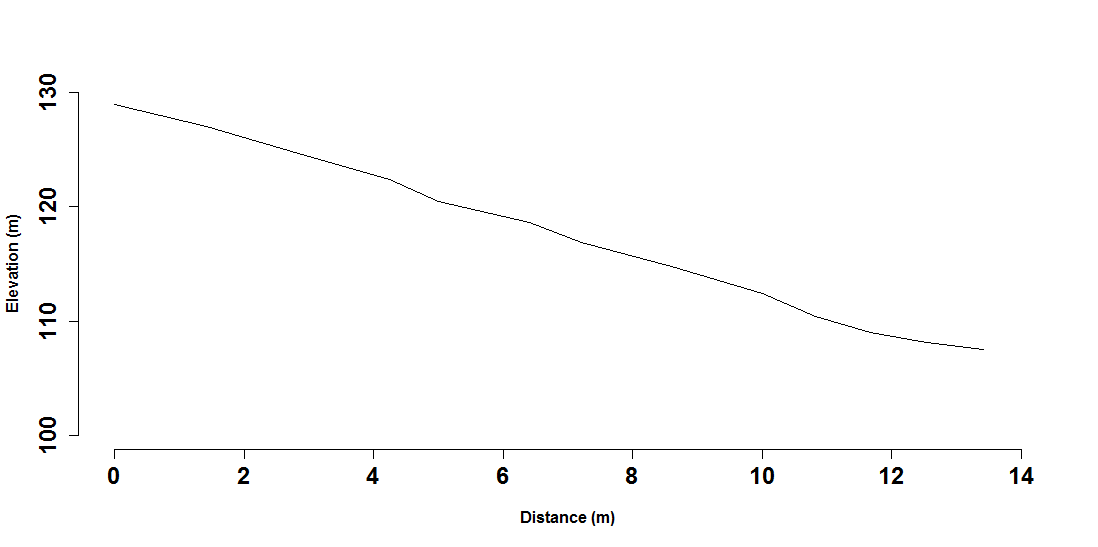
Finally we can plot the transect. First lets calculate a distance relative to the top of the transect. After this we can generate a plot below.
    dist = sqrt((transect[1, 1] - transect[, 1])^2 + (transect[1, 2] - transect[, 2])^2)
    plot(dist, transect[, 3], type = "l", xlab = "Distance (m)", ylab = "Elevation (m)")
So let’s take this a step further and consider the idea of a random toposequence. In reality, water does not only flow in the steepest direction, water can potentially move down to any lower elevation. And, a toposequence does not necessarily start at the highest elevation either. We can generate a random toposequence (Odgers, McBratney, and Minasny 2008), where we select a random point in the landscape, then find a random path to the top and bottom of a hillslope. In addition to the downhill routine, we need an uphill routine too.
The algorithm for the random toposequence could be written as:
-
Select a random point from a DEM.
-
Travel uphill:
a. Determine its 3 x 3 neighbor, and determine whether there are higher points? b. If yes, select randomly a higher point, add to the uphill sequence, and repeat step 2a. If this point is the highest, the uphill sequence ended.
- Travel downhill:
a. Determine its 3 x 3 neighbor, and determine whether there are lower points? b. If yes, select randomly a lower point, add to the downhill sequence, and repeat step 3a. If this point is the lowest or reached a stream, the downhill sequence ended.
From this algorithm plan, we need to specify two functions, one that
allows the transect to travel uphill and another which allows it to
travel downhill. For the one to travel downhill, we could use the
function from before find_steepest, but we want to build on that
function by allowing the user to indicate whether they want a randomly
selected smaller values, or whether they want to minimum every time.
Subsequently the 2 new functions would take the following form:
    travel_down <- function(dem, row_z, col_z, random) # function to simulate water moving down the slope input: dem and its row &
    # column random: TRUE use random path, FALSE for steepest path return:
    # row,col,z-z1 of lower neighbour
    {
        z1 = dem[row_z, col_z]
        # find its eight neighbour
        dir = c(-1, 0, 1)
        nr = nrow(dem)
        nc = ncol(dem)
        pz = matrix(data = NA, nrow = 3, ncol = 3)
        for (i in 1:3) {
            for (j in 1:3) {
                ro <- row_z + dir[i]
                co <- col_z + dir[j]
                if (ro > 0 & co > 0 & ro < nr & co < nc) {
                    pz[i, j] = dem[ro, co]
                }
            }
        }
        pz[2, 2] = NA
        pz <- pz - z1  # difference with centre value

        min_pz <- which(pz < 0, arr.ind = TRUE)
        nlow <- nrow(min_pz)
        if (nlow == 0) {
            min_pz <- which(pz == min(pz, na.rm = TRUE), arr.ind = TRUE)
        } else {
            if (random) {
                # find random lower value
                ir <- sample.int(nlow, size = 1)
                min_pz <- min_pz[ir, ]
            } else {
                # find lowest value
                min_pz <- which(pz == min(pz, na.rm = TRUE), arr.ind = TRUE)
            }
        }
        row_min <- row_z + dir[min_pz[1]]
        col_min <- col_z + dir[min_pz[2]]
        z_min <- dem[row_min, col_min]
        retval <- c(row_min, col_min, min(pz, na.rm = TRUE))
        return(retval)
    }


    travel_up <- function(dem, row_z, col_z, random) # function to trace water coming from up hill input: dem and its row & column
    # random: TRUE use random path, FALSE for steepest path return: row,col,z-zi of
    # higher neighbour
    {
        z1 = dem[row_z, col_z]
        # find its eight neighbour
        dir = c(-1, 0, 1)
        nr = nrow(dem)
        nc = ncol(dem)
        pz = matrix(data = NA, nrow = 3, ncol = 3)
        for (i in 1:3) {
            for (j in 1:3) {
                ro <- row_z + dir[i]
                co <- col_z + dir[j]
                if (ro > 0 & co > 0 & ro < nr & co < nc) {
                    pz[i, j] = dem[ro, co]
                }
            }
        }
        pz[2, 2] = NA
        pz <- pz - z1  # difference with centre value

        max_pz <- which(pz > 0, arr.ind = TRUE)  # find higher pixel
        nhi <- nrow(max_pz)
        if (nhi == 0) {
            max_pz <- which(pz == max(pz, na.rm = TRUE), arr.ind = TRUE)
        } else {
            if (random) {
                # find random higher value
                ir <- sample.int(nhi, size = 1)
                max_pz <- max_pz[ir, ]
            } else {
                # find highest value
                max_pz <- which(pz == max(pz, na.rm = TRUE), arr.ind = TRUE)
            }
        }
        row_max <- row_z + dir[max_pz[1]]
        col_max <- col_z + dir[max_pz[2]]
        retval <- c(row_max, col_max, max(pz, na.rm = TRUE))
        return(retval)
    }
Now we can generate a random toposequence. We will use the same
topo_dem data as before. First we select a point at random using a
random selection of a row and column value. We use set.seed() to ensure results are identical in terms of random selection of the seed point.
    nr <- nrow(topo_dem)  # no. rows in a DEM
    nc <- ncol(topo_dem)  # no. cols in a DEM

    # start with a random pixel as seed point
    set.seed(1203)
    row_z1 <- sample.int(nr, 1)
    col_z1 <- sample.int(nc, 1)
We then can use the travel_up function to get our transect to go up
the slope.
    # Travel uphill seed point as a starting point
    t <- 1
    transect_up <- matrix(data = NA, nrow = 100, ncol = 3)
    row_z <- row_z1
    col_z <- col_z1
    z1 = topo_dem[row_z, col_z]
    transect_up[t, 1] = row_z
    transect_up[t, 2] = col_z
    transect_up[t, 3] = z1

    highest = FALSE
    # iterate up the hill until highest point
    while (highest == FALSE) {
        result <- travel_up(dem = topo_dem, row_z, col_z, random = TRUE)
        if (result[3] <= 0)
            {
                highest == TRUE
                break
            }  # if found lowest point
        t <- t + 1
        row_z = result[1]
        col_z = result[2]
        z1 = topo_dem[row_z, col_z]
        transect_up[t, 1] = row_z
        transect_up[t, 2] = col_z
        transect_up[t, 3] = z1
    }
    transect_up <- na.omit(transect_up)
Next we then use the travel_down function to get our transect to go
down the slope from the seed point.
    # travel downhill create a data matrix to store results
    transect_down <- matrix(data = NA, nrow = 100, ncol = 3)
    # starting point
    row_z <- row_z1
    col_z <- col_z1
    z1 = topo_dem[row_z, col_z]  # a random pixel
    t <- 1
    transect_down[t, 1] = row_z
    transect_down[t, 2] = col_z
    transect_down[t, 3] = z1
    lowest = FALSE

    # iterate down the hill until lowest point
    while (lowest == FALSE) {
        result <- travel_down(dem = topo_dem, row_z, col_z, random = TRUE)
        if (result[3] >= 0)
            {
                lowest == TRUE
                break
            }  # if found lowest point
        t <- t + 1
        row_z = result[1]
        col_z = result[2]
        z1 = topo_dem[row_z, col_z]
        transect_down[t, 1] = row_z
        transect_down[t, 2] = col_z
        transect_down[t, 3] = z1
    }
    transect_down <- na.omit(transect_down)
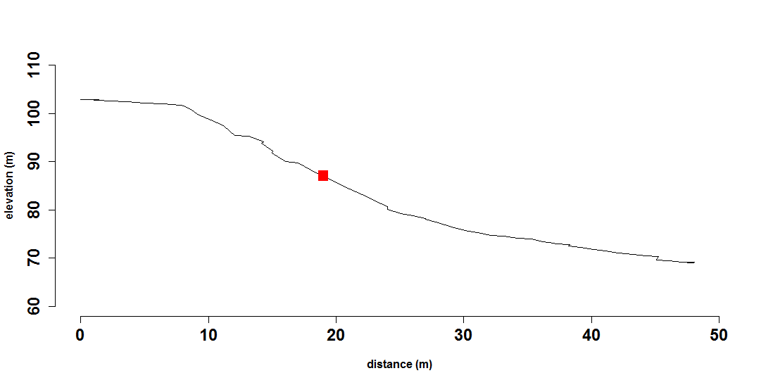
The idea then is to bind both uphill and downhill transects into a
single one. Note we are using the rbind function for this.
Furthermore, we are also using the order function here to re-arrange
the uphill transect so that the resultant binding will be sequential
from highest to lowest elevation. Finally, we then calculate the
distance relative to the hilltop.
    transect <- rbind(transect_up[order(transect_up[, 3], decreasing = T), ], transect_down[-1,
        ])

    # calculate distance from hilltop
    dist = sqrt((transect[1, 1] - transect[, 1])^2 + (transect[1, 2] - transect[, 2])^2)
The last step is to make the plot of the transect. We can also add the randomly selected seed point for visualization purposes.
    plot(dist, transect[, 3], type = "l", col = "red", xlim = c(0, 100), ylim = c(50,
        120), xlab = "Distance (m)", ylab = "Elevation (m)")

    points(dist[nrow(transect_up)], transect[nrow(transect_up), 3])
Exercises
After seeing how this algorithm works, you can modify the script to take in stream networks, and make the toposequence end once it reaches the stream. You can also add error trapping to handle missing values, and also in case where the downhill routine ends up in a local depression. This algorithm also can be used to calculate slope length, distance to a particular landscape feature (e.g. hedges), and so on.
References
Odgers, N P, A B McBratney, and B. Minasny. 2008. “Generation of Kth-Order Random Toposequences.” Computers & Geosciences 34 (5): 479–90.