CODE:
Get the code used for this section here
Uncertainty estimation based on local errors and fuzzy clustering
- Pre-work reading
- Data preparation
- Predictive model fitting
- Estimating underlying model errors
- Fuzzy clustering with extragrades
- Evaluating the quantification of uncertainties
- Mapping predictions and model uncertainties
- References
Pre-work reading
Similar to the uncertainty estimation based on local errors and data partitioning approach, the approach used in this example is similar in that uncertainty is expressed in the form of quantiles of the underlying distribution of model errors (residuals).
It contrasts however in terms of how the environmental data are treated. For the data partitioning approach, the method was based upon the hard classification defined by the partitions made in the covariates through the definition of the cubist model rulesets. The approach followed in this example uses a fuzzy clustering method of partition.
Essentially the approach is based on previous research by Shrestha and Solomatine (2006) where the idea is to partition a feature space into clusters (with a fuzzy k-means routine) which share similar model errors. A prediction interval (PI) is constructed for each cluster on the basis of the empirical distribution of residual observations that belong to each cluster. A PI is then formulated for each observation in the feature space according to the grade of their memberships to each cluster.
Shrestha and Solomatine (2006) applied this methodology to artificial and real hydrological data sets and it was found to be superior to other methods which estimate a PI. The Shrestha and Solomatine (2006) approach computes the PI independently and while free of the prediction model structure, it requires only the model or prediction outputs. Tranter et al. (2010) extended this approach to deal with observations that are outside of the training domain.
The method presented in this exercise was introduced by Malone et al. (2011) which modifies slightly the Shrestha and Solomatine (2006) and Tranter et al. (2010) approachesto enable it for a DSM framework. The approach is summarized by the flow diagram on the Figure below.
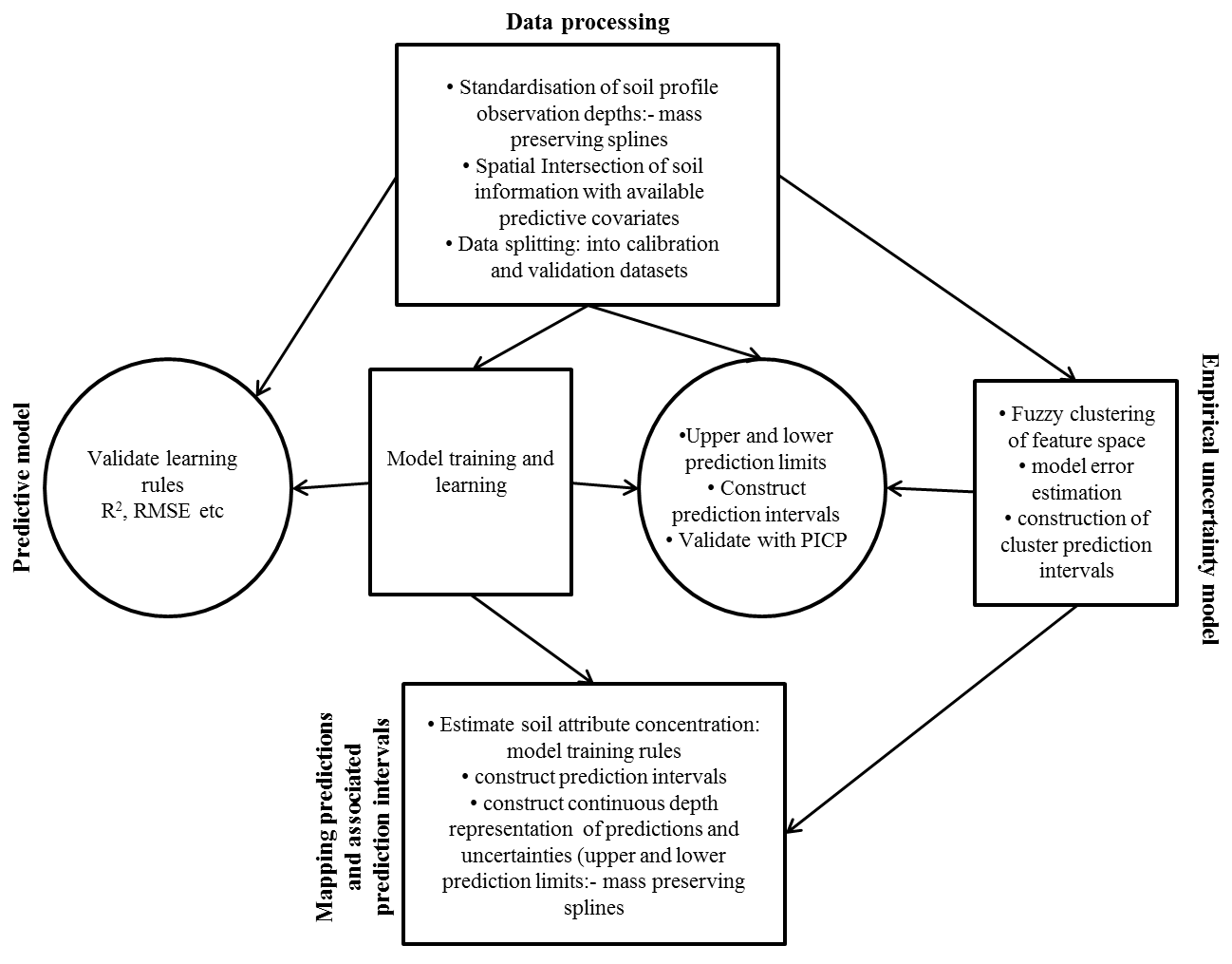
One benefit of using a fuzzy kmeans approach is that the spatial distribution of uncertainty is represented as a continuous variable. Further, the incorporation of extragrades in the fuzzy kmeans classifying provides an explicit means to identify and highlight areas of the greatest uncertainty and possibly where new sampling efforts should be prioritized. As shown in the figure the approach entails 3 main processes:
- Calibrating the spatial model
- deriving the uncertainty model which includes both estimations of model errors and fuzzy kmeans with extragrades classification
- Creation of maps of both spatial soil predictions and uncertainties.
Naturally, this framework is evaluated using an out-of-bag or better still, independent data set.
Data preparation
Here we will use a random forest regression kriging model for the prediction of soil pH across the study area. This model will also be incorporated into the uncertainty model via leave-one-out cross validation in order to derive the underlying model errors. As with other examples, we begin by preparing the data.
# Libraries
# may need to install the fuzme R package
# install.packages('devtools') library(devtools)
# install_bitbucket('brendo1001/fuzme/rPackage/fuzme')
library(ithir)
library(sf)
library(terra)
library(randomForest)
library(gstat)
library(fuzme)

# point data
data(HV_subsoilpH)

# Start afresh round pH data to 2 decimal places
HV_subsoilpH$pH60_100cm <- round(HV_subsoilpH$pH60_100cm, 2)

# remove already intersected data
HV_subsoilpH <- HV_subsoilpH[, 1:3]

# add an id column
HV_subsoilpH$id <- seq(1, nrow(HV_subsoilpH), by = 1)

# re-arrange order of columns
HV_subsoilpH <- HV_subsoilpH[, c(4, 1, 2, 3)]

# Change names of coordinate columns
names(HV_subsoilpH)[2:3] <- c("x", "y")
# save a copy of coordinates
HV_subsoilpH$x2 <- HV_subsoilpH$x
HV_subsoilpH$y2 <- HV_subsoilpH$y

# convert data to sf object
HV_subsoilpH <- sf::st_as_sf(x = HV_subsoilpH, coords = c("x", "y"))

# grids (covariate rasters from ithir package)
hv.sub.rasters <- list.files(path = system.file("extdata/", package = "ithir"), pattern = "hunterCovariates_sub",
full.names = TRUE)

# read them into R as SpatRaster objects
hv.sub.rasters <- terra::rast(hv.sub.rasters)

# extract covariate data
DSM_data <- terra::extract(x = hv.sub.rasters, y = HV_subsoilpH, bind = T, method = "simple")
DSM_data <- as.data.frame(DSM_data)

# check for NA values
which(!complete.cases(DSM_data))

## integer(0)

DSM_data <- DSM_data[complete.cases(DSM_data), ]

# subset data for modeling
set.seed(123)
training <- sample(nrow(DSM_data), 0.7 * nrow(DSM_data))
DSM_data_cal <- DSM_data[training, ]
DSM_data_val <- DSM_data[-training, ]
Predictive model fitting
Now we fit a random forest model using all possible covariates.
## Model fitting
hv.RF.Exp <- randomForest(x = DSM_data_cal[, 5:15], y = DSM_data_cal$pH60_100cm, data = DSM_data_cal, importance = TRUE, ntree = 500)

# goodness of fit on calibration data
goof(observed = DSM_data_cal$pH60_100cm, predicted = predict(hv.RF.Exp, newdata = DSM_data_cal), plot.it = FALSE)

##          R2 concordance       MSE      RMSE        bias
## 1 0.9230237   0.8855885 0.2841076 0.5330174 0.004619073
The hv.RF.Exp model appears to perform quite well when we examine the goodness of fit statistics.
Now we can examine the model residuals for any presence of spatial structure with variogram modeling. For the output below it does seems that there is some useful correlation structure in the residuals that will likely help to improve upon the performance of the hv.RF.Exp
model.
# calculate the residual
DSM_data_cal$residual <- DSM_data_cal$pH60_100cm - predict(hv.RF.Exp, newdata = DSM_data_cal)

# calculate empirical variogram of residuals
names(DSM_data_cal)[3:4] <- c("x", "y")
vgm1 <- variogram(residual ~ 1, ~x + y, data = DSM_data_cal, width = 200, cutoff = 3000)

# initialise variogram model parameters
mod <- vgm(psill = var(DSM_data_cal$residual), "Sph",  range = 3000, nugget = 0)

# fit variogram model
model_1 <- fit.variogram(vgm1, mod)
model_1

##   model     psill    range
## 1   Nug 0.2000183    0.000
## 2   Sph 0.0985494 1233.341

# variogram object
gR <- gstat(NULL, "hunterpH_residual_RF", residual ~ 1, data = DSM_data_cal, locations = ~x + y, model = model_1)
Estimating underlying model errors
We now need to estimate the model errors and a good way to do this is via the LOCV approach. To save time and get more quickly through the exercise the data out from below can be downloaded here.
## LEAVE - ONE - OUT - CROSS - VALIDATION estimation of empirical model
## residuals Note: the following step could take a little time to compute.
## This data can be loaded to avoid the following step of LOCV Just get your
## file paths right looResidualdata DSM_data_cal<-
## read.csv(file='hunter_DSMDat.csv') End note

# placeholder for cv residuals
DSM_data_cal$looResiduals <- NA

for (i in 1:nrow(DSM_data_cal)) {
  # subset model frame
  sub.frame <- DSM_data_cal[-i, ]
  # fit model
  looRFPred <- randomForest(x = sub.frame[, 5:15], y = sub.frame$pH60_100cm, importance = TRUE, ntree = 500)
  rf.preds <- predict(looRFPred, newdata = sub.frame[, 5:15])
  sub.frame$locv_resid <- sub.frame$pH60_100cm - rf.preds
  # residual variogram
  vgm.locv <- variogram(locv_resid ~ 1, ~x + y, data = sub.frame, width = 200, cutoff = 3000)
  mod.locv <- vgm(psill = var(sub.frame$locv_resid), "Sph", range = 3000, nugget = 0)
  model.locv <- fit.variogram(vgm.locv, mod.locv)
  # interpolate residual
  int.resids <- krige(locv_resid ~ 1, locations = ~x + y, data = sub.frame, newdata = DSM_data_cal[i, ], model = model.locv, debug.level = 0)[1, 3]
  looPred <- predict(object = looRFPred, newdata = DSM_data_cal[i, 5:15])
  DSM_data_cal$looResiduals[i] <- DSM_data_cal$pH60_100cm[i] - (looPred + int.resids)
  print(nrow(DSM_data_cal) - i)}
Fuzzy clustering with extragrades
The defining aspect of this uncertainty approach is fuzzy clustering with extragrades. McBratney and Gruijter (1992) recognized a limitation of the normal fuzzy clustering algorithm in that it had an inability to distinguish between observations very far from the cluster centroids and those at the centre of the centroid configuration. These observations were termed extragrades as opposed to intragrades, which are the observations that lie between the main clusters. The extragrades are considered the outliers of the data set and have a distorting influence on the configuration of the main clusters (Lagacherie et al. 1997). McBratney and Gruijter (1992) developed an adaptation to the FKM algorithm which distinguishes observations that should belong to an extragrade cluster. The FKM with extragrades algorithm minimizes the objective function:
where C is the c × p matrix of cluster centers where c is the cluster and p is the number of variables. M is the n × c matrix of partial memberships, where n is the number of observations; mijϵ is the partial membership of the ith observation to the jth cluster. ψ ≥ 1 is the fuzziness exponent. The square distance between the ith observation to the jth cluster is dij2. mi⋆ψ denotes the membership to the extragrade cluster. This function also requires the parameter alpha (α) to be defined, which is used to evaluate membership to the extragrade cluster.
A very good stand-alone software developed by Minasny (2002) called Fuzme contains the FKM with extragrades method, plus other clustering methods. The software may be downloaded for free from here.
The source script to this software has also been written to an R package of the same name.
Normally, the stand-alone software would be used because it is computationally much faster. However, using the fuzme package allows one to easily integrate the clustering procedures into a standard R workflow. For example, one of the issues of clustering procedures is the uncertainty regarding the selection of an optimal cluster number for a given data set.
There are a number of ways to determine an optimal solution. Some popular approaches include to determining the cluster combination which minimizes the Fuzzy Performance Index (FPI) or Modified partition Entropy (MPE). The MPE establishes the degree of fuzziness created by a specified number of clusters for a defined exponent value. The notion is that the smaller the MPE, the more suitable is the corresponding number of clusters at the given exponent value. A more sophisticated analysis is to look at the derivative of Je(C,M) with respect to ψ and is used to simultaneously establish the optimal ψ and cluster size. More is discussed about each of these indices by Odeh et al. (1992) and Bragato (2004).
The key generally is to define clusters which can be easily distinguished compared to a collection of clusters that are all quite similar. Such diagnostic criteria are useful; however it would be more beneficial to determine an optimal cluster configuration based on criteria that are meaningful to the current situation of deriving prediction uncertainties.
In this case we might want to evaluate the optimal cluster number and fuzzy exponent that maximizes the fidelity of PICP to confidence interval, and minimizes the prediction interval range. The idea here is to determine an optimal cluster number and fuzzy exponent based on criteria related to prediction interval width and PICP, together with some of the other fuzzy clustering criteria.
Optimization of the fuzzy classification parameters is no simple computational task and requires something akin the a grid search to find the best configuration setting whichever method is used.
The example below runs with a set of parameters that have been somewhat optimized offline. For you own data sets the optimization while time consuming is a necessary requirement of using this type of uncertainty quantification approach.
We essentially want to perform fuzzy clustering with extragrades upon the environmental covariate of the data points in the DSM_data_cal object. Fuzzy clustering with extragrades is implemented via a two-step procedure using the fobjk and fkme functions from the fuzme package.
The fobjkfunction allows one to find an optimal solution for alpha (α) which is the parameter that allows one to control the membership of data to the extragrade cluster. For example, if we wanted to stipulate that we want the average extragrade membership of a data set to be 10%, then we need to find an optimal solution for alpha to achieve that outcome. This can be controlled through the Uereq parameter of the fobjk function.
Now we need to prepare the data for clustering, and parameterize the other inputs of the function. The other inputs are: nclass, which is the number of clusters you want to define. Note that an extra cluster will be defined as this will be the extragrade cluster and the associated memberships. data is the data needed for clustering, U is an initial membership matrix in order to get the fuzzy clustering algorithm operable. phi is the fuzzy exponent, while distype refers to the distance metric to be used for clustering. There are 3 possible distance metrics available. These are: Euclidean (1), Diagonal (2), and Mahalanobis (3).
As an example of using the fobjk lets define 4 clusters with a fuzzy exponent of 1.2, and with the average extragrade membership of 10%. Currently this function is pretty slow to compute the optimal alpha, so be prepared to wait a while. Alternatively, the standalone Fuzme software described earlier makes this task more efficient.
## FUZZY KMEANS with EXTRAGRADES Computation of optimal alfa value used for FKM
## with extragrades Note: the following step could take a little time to compute.  End Note

data.t <- DSM_data_cal[, 5:15]  # data to be clustered
nclass.t <- 4  # number of clusters
phi.t <- 1.2  # fuzzy exponent
distype.t <- 3  # 3 = Mahalanobis distance
Uereq.t <- 0.1  # average extragrade membership

# initial membership matrix
scatter.t <- 0.2  # scatter around initial membership
ndata.t <- dim(data.t)[1]
U.t <- fuzme::initmember(scatter = scatter.t, nclass = nclass.t, ndata = ndata.t)

# run fuzzy objective function
alfa.t <- fuzme::fobjk(Uereq = Uereq.t, nclass = nclass.t, data = data.t, U = U.t,
phi = phi.t, distype = distype.t)
alfa.t
Remember the fobjk function will only return the optimal alfa value which in this particular case was 0.01136809. This value then gets inserted into the associated fkme function in order to estimate the memberships of the data to each cluster and the extragrade cluster. The fkme function also returns the cluster centroids too which are critical to the work need for allocation of memberships to new data cases.
The fkme function is parameterized similarly to fobjk, yet with some additional inputs related to the number of allowable iterations for convergence (maxiter), the convergence criterion value (toldif), and whether or not to display behind-the-scenes processing.
While the below is useful to watch as it works to minimise the objective function, it does require some time to converge. If needed you can avoid this step and load directly the expected output from below.
## FKM with extragrade Note: the following step could take a little time to
## compute.  This data can be loaded to avoid the following step of FKM with
## extragrade Just get your file paths right readRDS(file =
## 'fkme_example_out.rds') [download link] End Note

alfa.t <- 0.01136809
tester <- fkme(nclass = nclass.t, data = data.t, U = U.t, phi = phi.t, alfa = alfa.t,
maxiter = 500, distype = distype.t, toldif = 0.01, verbose = 1)
The fkme function returns a list with a number of elements. At this stage we are primarily interested in the elements membership and centroid which we will use a little later on.
As described earlier, there are a number of criteria to assess the validity of a particular clustering configuration. We can evaluate these by using the fvalidity function. It essentially takes in a few of the outputs from the fkme function.
## Fuzzy performance indices
fuzme::fvalidity(U = tester$membership[, 1:4],
dist = tester$distance,
centroid = tester$centroid,
nclass = 4,
phi = 1.2,
W = tester$distNormMat)

##         fpi       mpe         S   dJ/dphi
## 1 0.5186971 0.4136468 0.9024766 -1808.337
Another useful metric is the confusion index (after Burrough et al. (1997)) which in our case looks at the similarity between the highest and second highest cluster memberships. The confusion index is estimated for each data point. Taking the average over the data set provides some sense of whether cluster can be distinguished from each other.
## Confusion index
mean(confusion(nclass = 5, U = tester$membership))

## [1] 0.3499941


# Note number of cluster is set to 5 to account for the Additional extragrade cluster.
We now need to assign each data point a one of the clusters we have derived. The assignment is based on the cluster which has the highest membership grade.
## Assign class for each point
membs <- as.data.frame(tester$membership)
membs$class <- NA
for (i in 1:nrow(membs)) {
  mbs2 <- membs[i, 1:ncol(tester$membership)]
  # which is the maximum probability on this row
  membs$class[i] <- which(mbs2 == max(mbs2))[1]}

membs$class <- as.factor(membs$class)
summary(membs$class)

##  1  2  3  4  5
## 96 75 58 87 38

# combine with main data frame that cotain LOCV model residuals
DSM_data_cal <- cbind(DSM_data_cal, membs$class)
names(DSM_data_cal)[ncol(DSM_data_cal)] <- "class"
Then we derive the cluster model error. This entails splitting the DSM_data_cal object up on the basis of the cluster with the highest membership i.e. DSM_data_cal$class.
## QUANTILES OF RESIDUALS IN EACH CLASS FOR CLASS PREDICTION LIMITS
DSM_data_cal.split <- split(DSM_data_cal, DSM_data_cal$class)

# cluster lower prediction limits
quanMat1 <- matrix(NA, ncol = 10, nrow = length(DSM_data_cal.split))
for (i in 1:length(DSM_data_cal.split)) {
quanMat1[i, ] <- quantile(DSM_data_cal.split[[i]][, "looResiduals"], probs = c(0.005, 0.0125, 0.025, 0.05, 0.1, 0.2, 0.3, 0.4, 0.45, 0.475), na.rm = FALSE, names = F, type = 7)}

row.names(quanMat1) <- levels(DSM_data_cal$class)
quanMat1[nrow(quanMat1), ] <- quanMat1[nrow(quanMat1), ] * 2
quanMat1 <- t(quanMat1)
row.names(quanMat1) <- c(99, 97.5, 95, 90, 80, 60, 40, 20, 10, 5)

# cluster upper prediction limits
quanMat2 <- matrix(NA, ncol = 10, nrow = length(DSM_data_cal.split))
for (i in 1:length(DSM_data_cal.split)) {
  quanMat2[i, ] <- quantile(DSM_data_cal.split[[i]][, "looResiduals"], probs = c(0.995, 0.9875, 0.975, 0.95, 0.9, 0.8, 0.7, 0.6, 0.55, 0.525), na.rm = FALSE, names = F, type = 7)}

quanMat2[quanMat2 < 0] <- 0
row.names(quanMat2) <- levels(DSM_data_cal$class)
quanMat2[nrow(quanMat2), ] <- quanMat2[nrow(quanMat2), ] * 2
quanMat2 <- t(quanMat2)
row.names(quanMat2) <- c(99, 97.5, 95, 90, 80, 60, 40, 20, 10, 5)
The objects quanMat1 and quanMat2 represent the lower and upper model errors for each cluster for each quantile respectively.
For the extragrade cluster, we multiple the error by a constant, here 2, in order to explicitly indicate that the extragrade cluster (being outliers of the data) have a higher uncertainty.
Evaluating the quantification of uncertainties
Using the out-of-bag data, we need evaluate the PICP and prediction interval width. This requires first allocating cluster memberships to the points on the basis of outputs from using the fkme function, then using these together with the cluster prediction limits to evaluate weighted averages of the prediction limits for each point. With that done we can then derive the unique upper and lower prediction interval limits for each point at each confidence level.
First, for the membership allocation, we use the fuzExall function. Essentially this function takes in outputs from the fkme function and in our case, specifically that concerning the tester object. Recall that the out-of-bag data is saved to the DSM_data_val object.
## Evaluation of predictions and uncertainties with out of bag data covariates
## of the out-of-bag data
vCovs <- DSM_data_val[, 5:15]

# run fkme allocation function
fuzAll <- fuzme::fuzExall(data = vCovs,
phi = 1.2,
centroid = tester$centroid,
distype = 3,
W = tester$distNormMat,
alfa = tester$alfa)

# Get the memberships
fuz.me <- fuzAll$membership
A “fuzzy committee” approach is used to estimate the underlying residual at each point. In this case the upper and lower limits are derived by weighted mean of the lower and upper model errors of each cluster, where the weights are the cluster memberships. This can be defined mathematically as:
where PIiL and
PIiU correspond to the weighted lower and upper limits for the i th observation. PICjL and PICjU are the lower and upper limits for each cluster j, and mij is the membership grade of the ith observation to cluster j (which were derived in the previous step). In R, this can be interpreted as:
# lower prediction limit
lPI.mat <- matrix(NA, nrow = nrow(fuz.me), ncol = 10)
for (i in 1:nrow(lPI.mat)) {
  for (j in 1:nrow(quanMat1)) {
    lPI.mat[i, j] <- sum(fuz.me[i, 1:ncol(fuz.me)] * quanMat1[j, ])}}

# upper prediction limit
uPI.mat <- matrix(NA, nrow = nrow(fuz.me), ncol = 10)
for (i in 1:nrow(uPI.mat)) {
  for (j in 1:nrow(quanMat2)) {
    uPI.mat[i, j] <- sum(fuz.me[i, 1:ncol(fuz.me)] * quanMat2[j, ])}}
Then we want to add these values to the actual regression kriging predictions.
# Regression kriging predictions for out-of-bag data
names(DSM_data_val)[3:4] <- c("x", "y")
DSM_data_val$rf_preds <- predict(object = hv.RF.Exp, newdata = DSM_data_val[, 5:15])
DSM_data_val$krig_res <- krige(residual ~ 1, data = DSM_data_cal, locations = ~x + y, model = model_1, newdata = DSM_data_val)[, 3]

DSM_data_val$RK_preds <- DSM_data_val$rf_preds + DSM_data_val$krig_res

# evaluation of model goodness of fit
goof(observed = DSM_data_val$pH60_100cm, predicted = DSM_data_val$RK_preds, plot.it = FALSE)

##          R2 concordance      MSE    RMSE       bias
## 1 0.2972396   0.4165083 1.348223 1.16113 0.04220921

# Derive validation lower prediction limits
lPL.mat <- matrix(NA, nrow = nrow(fuz.me), ncol = 10)
for (i in 1:ncol(lPL.mat)) {
  lPL.mat[, i] <- DSM_data_val$RK_preds + lPI.mat[, i]}

# Derive validation upper prediction limits
uPL.mat <- matrix(NA, nrow = nrow(fuz.me), ncol = 10)
for (i in 1:ncol(uPL.mat)) {
  uPL.mat[, i] <- DSM_data_val$RK_preds + uPI.mat[, i]}
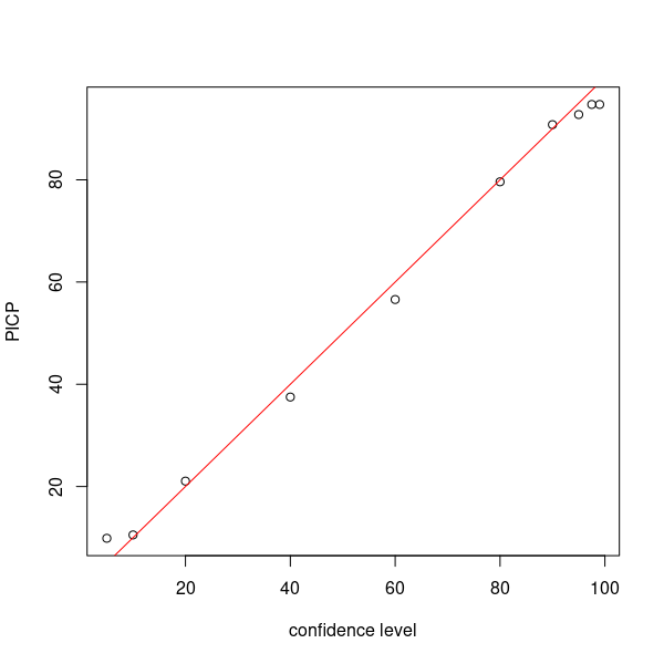
Now as in the previous uncertainty approaches we estimate the PICP for each level of confidence. We can also estimate the average prediction interval length too. We will do this for the 90% confidence level.
## PICP
bMat <- matrix(NA, nrow = nrow(fuz.me), ncol = 10)
for (i in 1:10) {
  bMat[, i] <- as.numeric(DSM_data_val$pH60_100cm <= uPL.mat[, i] & DSM_data_val$pH60_100cm >= lPL.mat[, i])}

# make plot
par(mfrow = c(1, 1))
cs <- c(99, 97.5, 95, 90, 80, 60, 40, 20, 10, 5)
plot(cs, ((colSums(bMat)/nrow(bMat)) * 100), ylab = "PICP", xlab = "confidence level")
# draw 1:1 line
abline(a = 0, b = 1, col = "red")

# prediction interval width (averaged)
as.matrix(mean(uPL.mat[, 4] - lPL.mat[, 4]))

##          [,1]
## [1,] 3.947908
Mapping predictions and model uncertainties
With the spatial model defined together with the fuzzy clustering with the associated parameters and model errors, we can create the associated maps. First, the random forest regression kriging map.
## MAPPING random forest model extension
map.Rf <- terra::predict(object = hv.sub.rasters, model = hv.RF.Exp, na.rm = TRUE)

# kriged residuals
map.KR <- terra::interpolate(object = hv.sub.rasters, model = gR, xyOnly = TRUE)

# combine
map.final <- map.Rf + map.KR[[1]]
Now we need to map the prediction intervals. Essentially for every pixel on the map we first need to estimate the membership value to each cluster. This membership is based on a distance of the covariate space and the centroids of each cluster. To do this we use the fuzzy allocation function (fuzExall) that was used earlier. This time we use the fuzzy parameters from the tester object. We need to firstly create a data.frame from the stack of covariates.
# Prediction Intervals
# get rasters into a data frame to advance calculation of memberships

hunterCovs.df <- data.frame(cellNos = seq(1:ncell(hv.sub.rasters)))
vals <- as.data.frame(terra::values(hv.sub.rasters))
hunterCovs.df <- cbind(hunterCovs.df, vals)
hunterCovs.df <- hunterCovs.df[complete.cases(hunterCovs.df), ]
cellNos <- c(hunterCovs.df$cellNos)
gXY <- data.frame(terra::xyFromCell(hv.sub.rasters, cellNos))
hunterCovs.df <- cbind(gXY, hunterCovs.df)
Now we prepare all the other inputs for the fuzExall function, and then run it. This may take a little time.
fuz.me_ALL <- fuzExall(
data = hunterCovs.df[, 4:ncol(hunterCovs.df)],
centroid = tester$centroid,
phi = 1.2,
distype = 3,
W = tester$distNormMat,
alfa = tester$alfa)
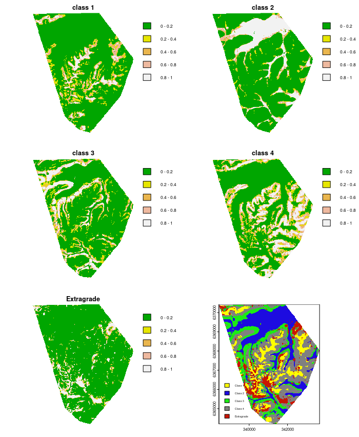
With the memberships estimated, lets visualize them by creating the associated membership maps
# attribute class allocation to maximum membership
membs.table <- as.data.frame(fuz.me_ALL$membership)
membs.table$class <- NA
for (i in 1:nrow(membs.table)) {
  mbs2 <- membs.table[i, 1:5]
  # which is the maximum probability on this row
  membs.table$class[i] <- which(mbs2 == max(mbs2))[1]}

# combine coordinates to memberships
hvCovs <- cbind(hunterCovs.df[, 1:2], membs.table)

# Create rasters of memberships and class
map.class1mem <- terra::rast(hvCovs[, c(1, 2, 3)], type = "xyz")
names(map.class1mem) <- "class_1"
map.class2mem <- terra::rast(hvCovs[, c(1, 2, 4)], type = "xyz")
names(map.class2mem) <- "class_2"
map.class3mem <- terra::rast(hvCovs[, c(1, 2, 5)], type = "xyz")
names(map.class3mem) <- "class_3"
map.class4mem <- terra::rast(hvCovs[, c(1, 2, 6)], type = "xyz")
names(map.class4mem) <- "class_4"
map.classExtramem <- terra::rast(hvCovs[, c(1, 2, 7)], type = "xyz")
names(map.classExtramem) <- "class_ext"
map.class <- terra::rast(hvCovs[, c(1, 2, 8)], type = "xyz")
names(map.class) <- "class"

## PLOTTING
par(mfrow = c(3, 2))
plot(map.class1mem, main = "class 1", col = terrain.colors(length(seq(0, 1, by = 0.2)) - 1), axes = FALSE, breaks = seq(0, 1, by = 0.2))
plot(map.class2mem, main = "class 2", col = terrain.colors(length(seq(0, 1, by = 0.2)) - 1), axes = FALSE, breaks = seq(0, 1, by = 0.2))
plot(map.class3mem, main = "class 3", col = terrain.colors(length(seq(0, 1, by = 0.2)) - 1), axes = FALSE, breaks = seq(0, 1, by = 0.2))
plot(map.class4mem, main = "class 4", col = terrain.colors(length(seq(0, 1, by = 0.2)) - 1), axes = FALSE, breaks = seq(0, 1, by = 0.2))
plot(map.classExtramem, main = "Extragrade", col = terrain.colors(length(seq(0, 1, by = 0.2)) - 1), axes = FALSE, breaks = seq(0, 1, by = 0.2))
levels(map.class) = data.frame(value = 1:5, desc = c("Class 1", "Class 2", "Class 3", "Class 4", "Extragrade"))
area_colors <- c("#FFFF00", "#1D0BE0", "#1CEB15", "#808080", "#C91601")
plot(map.class, col = area_colors, plg = list(loc = "bottomleft", cex = 0.6))
The last mapping task is to evaluate the 90% prediction intervals. Again we use the fuzzy committee approach given the cluster memberships and the cluster model error limits.
# Mapping of upper and lower predicition limits Lower limits for each class
quanMat1["90", ]

##         1         2         3         4         5
## -1.609167 -1.949015 -1.805720 -1.452031 -2.495811

# upper limits for each class
quanMat2["90", ]

##        1        2        3        4        5
## 2.060832 2.288711 2.340094 1.775154 3.330916
Now we perform the weighted averaging prediction.
# stack the rasters
s2 <- c(map.class1mem, map.class2mem, map.class3mem, map.class4mem, map.classExtramem)

# lower limit
f1 <- function(x) ((x[1] * quanMat1["90", 1]) + (x[2] * quanMat1["90", 2]) + (x[3] * quanMat1["90", 3]) + (x[4] * quanMat1["90", 4]) + (x[5] * quanMat1["90", 5])) mapRK.lower <- terra::app(x = s2, fun = f1)

# upper limit
f2 <- function(x) ((x[1] * quanMat2["90", 1]) + (x[2] * quanMat2["90", 2]) + (x[3] * quanMat2["90", 3]) + (x[4] * quanMat2["90", 4]) + (x[5] * quanMat2["90", 5])) mapRK.upper <- terra::app(x = s2, fun = f2)
And finally we can derive the upper and lower prediction limits.
## Final maps Lower prediction limit
map.final.lower <- map.final + mapRK.lower

# Upper prediction limit
map.final.upper <- map.final + mapRK.upper

# Prediction interval range
map.final.pir <- map.final.upper - map.final.lower
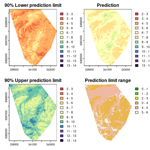
And now we can display the necessary maps:
# color ramp
phCramp <- c("#d53e4f", "#f46d43", "#fdae61", "#fee08b", "#ffffbf", "#e6f598", "#abdda4", "#66c2a5", "#3288bd", "#5e4fa2", "#542788", "#2d004b")

brk <- c(2:14)
par(mfrow = c(2, 2))
plot(mapRF.lowerPI, main = "90% Lower prediction limit", breaks = brk, col = phCramp)
plot(mapRF.fin, main = "Prediction", breaks = brk, col = phCramp)
plot(mapRF.upperPI, main = "90% Upper prediction limit", breaks = brk, col = phCramp)
plot(mapRF.PIrange, main = "Prediction limit range", col = terrain.colors(length(seq(0, 6.5, by = 1)) - 1), axes = FALSE, breaks = seq(0, 6.5, by = 1))
References
Bragato, G. 2004. “Fuzzy Continuous Classification and SpatialInterpolation in Conventional Soil Survey for Soil Mapping of the Lower Piave Plain.” Geoderma 118: 1–16.
Burrough, P. A, P. F. M van Gaans, and R Hootsmans. 1997. “Continuous Classifcation in Soil Survey: Spatial Correlation, Confusion and Boundaries.” Geoderma 77: 115–35.
Lagacherie, P., D. R. Cazemier, P. F. M. vanGaans, and P. A. Burrough. 1997. “Fuzzy k-Means Clustering of Fields in an Elementary Catchment and Extrapolation to a Larger Area.” Geoderma 77: 197–216.
Malone, B P, A B McBratney, and B Minasny. 2011. “Empirical Estimates of Uncertainty for Mapping Continuous Depth Functions of Soil Attributes.” Geoderma 160: 614–26.
McBratney, A. B., and J. J. de Gruijter. 1992. “Continuum Approach to Soil Classification by Modified Fuzzy k-Means with Extragrades.” Journal of Soil Science 43: 159–75.
Minasny, A. B., B McBratney. 2002. FuzME Version 3.0. Australian Centre for Precision Agriculture, The University of Sydney, Australia.
Odeh, I. O. A., A. B. McBratney, and D. J. Chittleborough. 1992. “Soil Pattern Recognition with Fuzzy-c-Means: Application to Classification and Soil-Landform Interrelationships.” Soil Science Society of America Journal 56: 506–16.
Shrestha, D. L, and D. P Solomatine. 2006. “Machine Learning Approaches for Estimation of Prediction Interval for the Model Output.” Neural Networks 19: 225–35.
Tranter, G., B. Minasny, and A. B. McBratney. 2010. “Estimating Pedotransfer Function Prediction Limits Using Fuzzy k-Means with Extragrades.” Soil Science Society of America Journal 74: 1967–75.