CODE:
Download the ea_ras_func function that works in conjuction with script
Customising public digital soil mapping products with mass preserving splines
- A background story of sorts about digital soil mapping and mass preserving splines
- Making use of publicly available digital soil maps and customizing them to suit your specific needs
Rscripting example of applying spline depth function directly to digital soil maps- A final word
There are now plenty of soil maps which digitally represent the soil variation across landscapes in both the lateral and vertical dimensions.
Some might say this is akin to digital twinning for natural resources. These representations are usually provided as depth slices or layers for specified depth intervals.
What is probably not as widely known or practiced is that one can use these data to generate custom soil maps (in terms of vertical support representation) according to the wishes of the end-user or map maker.
In this post, the mass-preserving spline is re-introduced not for harmonising soil profile data, but for creating user-defined soil maps that exploit 3D digital soil mapping information that are becoming widely available publicly and for free.
A background story of sorts about digital soil mapping and mass preserving splines
Go back to digital soil mapping course
There do not appear to be new official global activities associated with the GlobalSoilMap.net project (Sanchez et al. 2009) any longer.
This initiative was very active between 2009 and 2013 and created a flurry of efforts to map the world’s soils and their characteristics. The initial philosophy of GlobalSoilMap.net was for nodes to coordinate activities across a selected number of regions and individual countries would work within the nodes to develop digital soil mapping products for within country, and provide assistance to other countries in the region where the necessary digital soil mapping skill base was still in development.
Probably the greatest success and lasting legacy of the GlobalSoilMap.net project was the creation of a document that specified the expected outputs to be developed i.e. the GlobalSoilMap.net specifications (Arrouays et al. 2014). These specifications have guided digital soil mapping practices throughout the world since they were published. Global soil mapping efforts now are coordinated a little differently and mainly through the auspices of the Global Soil Parntership. One of the main GlobalSoilMap.net specifications was the requirement to produce maps for the following soil properties: SOC, clay, silt, sand and coarse fragment contents, pH, ECEC, soil depth and available depth to rooting, bulk density (whole soil and fine earth fraction), and available water capacity at standard depths to 2m. Specifically for the depth intervals of: 0-5cm, 5-15cm, 15-30cm, 30-60cm, 60-100cm, 100-200cm.
Early research was dedicated to figuring out approaches for generating digital maps for the specified standard depths given legacy soil profile data and the existing digital soil mapping techniques. The mass preserving spline (Bishop et al. 1999) became a critical methodological advancement in this regard as it enabled soil profile data all with disparate depth information to be harmonized. The spline was fitted to the soil profile data and this depth function is then integrated to get the target soil property values for the standard depths or any specified depth intervals or set of depth intervals according to the user.
The mass preserving spline is super useful and its mass preserving properties mean that the original soil profile information is never lost after the function is fitted. In a digital soil mapping context, first soil profile data is gathered, the splines are fitted individually to each profile from which the soil target variables at each standard depth is retrieved. Then spatial models are fitted for each depth using a collected suite of environmental covariate layers as predictor variables. This is the general approach undertaken in Malone et al. (2009) which has also been done too throughout the world.
While this approach remains popular, different 3D spatial modelling approaches have evolved (see for example Hengl (2017), Orton et al. (2016), and Poggio and Gimona (2014)). But ultimately, the end result from whatever approach is used are digital soil maps of specific variables at each standard depth.
In most cases, the depth support of these maps is supposedly representing an average of the specified target variable for the given standard depth.
What is observed throughout the world are a proliferation of digital soil maps, all produced in a way that meet or closely adhere to the specifications set out in Arrouays et al. (2014).
Australia is one of these places, and earlier efforts are described in Grundy et al. (2015). The great thing about this effort and more recent updates to The Soil and Landscape Grid of Australia (SLGA) is now these data are available for everyone to retrieve and importantly use for any number of purposes that requires spatial soil information. This data is easy to access and download. As can be observed, there are several ways in which this data can be retrieved.
Making use of publicly available digital soil maps and customizing them to suit your specific needs
How to make use of the available digital soil maps poses some a few considerations.
It is great to be able to have a 3-D digital representation of soils, in some ways akin to a digital twin. But without necessary tools with which to analyse the representations of these data i.e. interrogating and integrating the 0-5cm,5-15cm, 15-30cm, 30-60cm, 60-100cm, and 100-200cm layers, one will be limited in realising the utility of this information.
One tool to be described in this post is the mass-preserving spline which we were just introduced to earlier in regards to harmonising soil profile data.
Essentially the soil target variable data together with information about corresponding depths intervals are parameters of the spline. Therefore where there is layered and gridded digital soil maps we basically can fit a spline at each grid cell and then interrogate the fitted spline to generate new outputs at a different vertical support.
This allows one to customize their soil mapping information to a form that is conducive for their own particular needs. Furthermore a step forwards on this is that one can facilitate inferences as was exemplified in Malone et al. (2009) where variables such as depth to which carbon stocks breached a given threshold value, or estimated the water holding capacity to a given depth etc. One can even get more sophisticated around inference for such things as detecting depth to a texture contrast layer or to some given soil constraint.
The important key point here is that the layered 3D representation of soil information as specified for GlobalSoilMap or for any other similar product, is that there is added utility of this information beyond the base maps.
This post intends to exemplify the splines approach for 3D soil mapping products using some Version 2 SLGA digital soil maps.
At the moment the code for doing this comes from a bespoke R function
called
ea_ras_func.
For all intents and purposes, the function is the same as would be used
to fit to soil profile data but is modified slightly for grid data.
Another key point is that as there are no gaps between soil values as the layers are adjacent to one another, there is no interpolation, meaning that the mass-preserving properties of the spline are much easier to adhere to.
R scripting example of applying spline depth function directly to digital soil maps
For this example the only R package required is terra. Once you have
downloaded the ea_ras_func, you load this into R using the source
function. Note you will need to have the appropriate file paths when you
do the source.
library(terra)

# load spline raster function
source("ea_ras_func.R")
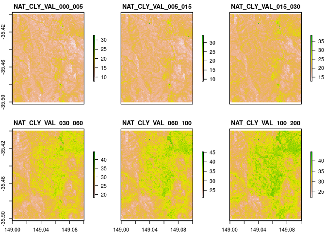
SLGA digital soil maps on the web are located at https://esoil.io/TERNLandscapes/Public/Products/TERN/SLGA/. In this particular example we want to get hold of the national coverage of soil clay content % for each of the soil depth intervals i.e. 0-5cm,5-15cm, 15-30cm, 30-60cm, 60-100cm, and 100-200cm. We are just after the estimated means here for each depth.
The really helpful feature of these large data sets are that they are stored as COGs or Cloud Optimised GeoTIFFs. As suggested, COGs are GeoTIFF files, but are internally formatted to allow efficient access to the raster data across the web. This means you can quickly and efficiently access and view large raster data sets over the web without having to download the entire data set locally. Portions of, or the entire data set, can also be downloaded as required.
# Download SLGA V2 mapping
SLGA_V2_clay <- c('/vsicurl/https://esoil.io/TERNLandscapes/Public/Products/TERN/SLGA/CLY/CLY_000_005_EV_N_P_AU_TRN_N_20210902.tif',
'/vsicurl/https://esoil.io/TERNLandscapes/Public/Products/TERN/SLGA/CLY/CLY_005_015_EV_N_P_AU_TRN_N_20210902.tif',
'/vsicurl/https://esoil.io/TERNLandscapes/Public/Products/TERN/SLGA/CLY/CLY_015_030_EV_N_P_AU_TRN_N_20210902.tif',
'/vsicurl/https://esoil.io/TERNLandscapes/Public/Products/TERN/SLGA/CLY/CLY_030_060_EV_N_P_AU_TRN_N_20210902.tif',
'/vsicurl/https://esoil.io/TERNLandscapes/Public/Products/TERN/SLGA/CLY/CLY_060_100_EV_N_P_AU_TRN_N_20210902.tif',
'/vsicurl/https://esoil.io/TERNLandscapes/Public/Products/TERN/SLGA/CLY/CLY_100_200_EV_N_P_AU_TRN_N_20210902.tif')

# load in rasters and stack
SLGA_V2_clay.stk <- terra::rast(SLGA_V2_clay)
SLGA_V2_clay.stk

## class       : SpatRaster
## dimensions  : 40800, 49200, 6  (nrow, ncol, nlyr)
## resolution  : 0.0008333333, 0.0008333333  (x, y)
## extent      : 112.9996, 153.9996, -44.00042, -10.00042  (xmin, xmax, ymin, ymax)
## coord. ref. : lon/lat WGS 84 (EPSG:4326)
## sources     : CLY_000_005_EV_N_P_AU_TRN_N_20210902.tif
##               CLY_005_015_EV_N_P_AU_TRN_N_20210902.tif
##               CLY_015_030_EV_N_P_AU_TRN_N_20210902.tif
##               ... and 3 more source(s)
## names       : CLY_0~10902, CLY_0~10902, CLY_0~10902, CLY_0~10902, CLY_0~10902, CLY_1~10902
There is an astounding amount of data readied for analysis. However, we only want a small bit and will therefore crop the national maps to a given area of interest which here is part of King Island an island in the Bass Strait off mainland Australia.
aoi <- terra::ext(149.00,149.1, -35.50, -35.40)
rc <- terra::crop(SLGA_V2_clay.stk, aoi)
Using the ea_rasSp function is relatively straightforward. Basically
it will only ingest a stacked set of rasters. The function automatically
assumes each raster layer represents a given depth interval or slice,
which could be GSM standard depths or some other representation. We
specify this with the dIn parameter where
dIn = c(0,5,15,30,60,100,200) corresponds to the GSM depths
i.e. 0-5cm, 5-15cm, 15-30cm, 30-60cm, 60-100cm and 100-200cm. dOut is
the parameter for the new depth intervals we want. Below we a signalling
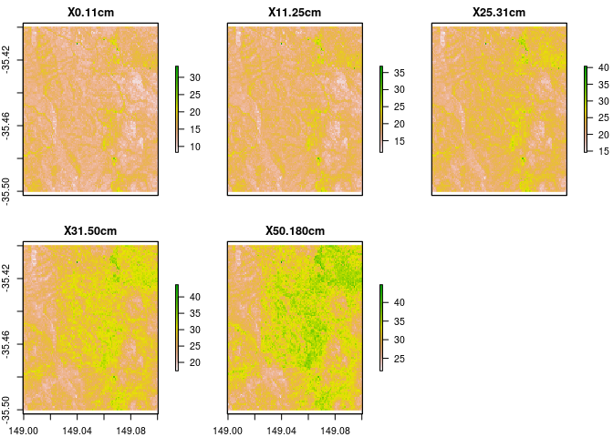
(just to be unusual) to get the 0-11cm, 11-25cm, 25-31cm, 21-50cm, and
50-180cm depth intervals. The vlow and vhigh parameters are for
constraining the spline fit to be within normal ranges which for soil
texture is between 0% and 100%. The other important parameter is lam
which determines the amount of flex in the fitted spline. The value 0.1
is usually a acceptable choice, but one can select their own choice
based on there own criteria. High values result in stiff splines while
low values result in flexible splines.
# use raster spline function with unusual depth interval outputs
rc.new<- ea_rasSp(obj= rc, # raster stack object
            lam = 0.1, # lambda
            # These are SLGA standard depths (but could be any depths though)
            dIn = c(0,5,15,30,60,100,200),
            # User specified depths
            dOut = c(0,11,25,31,50,180),
            vlow = 0,
            vhigh = 100,
            show.progress=FALSE)
rc.new

## class       : SpatRaster
## dimensions  : 120, 120, 5  (nrow, ncol, nlyr)
## resolution  : 0.0008333333, 0.0008333333  (x, y)
## extent      : 148.9996, 149.0996, -35.49958, -35.39958  (xmin, xmax, ymin, ymax)
## coord. ref. :
## source(s)   : memory
## names       :    0-11cm,   11-25cm,   25-31cm,   31-50cm, 50-180cm
## min values  :  4.978169,  6.295709,  8.102672,  9.760598, 18.10916
## max values  : 22.512454, 26.149973, 27.870316, 34.440504, 38.77937
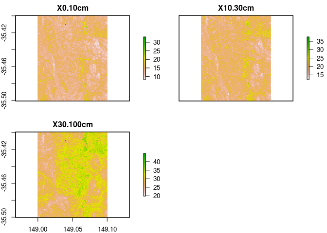
Probably a more usual thing to do might be to get to top 10cm, then 10-30cm, and finally 30-100cm.
# use raster spline function with less unusual depth interval outputs
rc.new2<- ea_rasSp(obj= rc, # raster stack object
          lam = 0.1, # lambda
          # These are SLGA standard depths (but could be any depths though)
          dIn = c(0,5,15,30,60,100,200),
          # User specified depths
          dOut = c(0,10,30,100),
          vlow = 0,
          vhigh = 100,
          show.progress=FALSE)

rc.new2

## class       : SpatRaster
## dimensions  : 120, 120, 3  (nrow, ncol, nlyr)
## resolution  : 0.0008333333, 0.0008333333  (x, y)
## extent      : 148.9996, 149.0996, -35.49958, -35.39958  (xmin, xmax, ymin, ymax)
## coord. ref. :
## source(s)   : memory
## names       :    0-10cm,   10-30cm, 30-100cm
## min values  :  4.963896,  6.665595, 10.70752
## max values  : 22.350791, 26.473108, 37.12655
A final word
The intention here was to illustrate that the outputs commonly generated in digital soil mapping that adhere the GSM specifications have much greater utility than just the standard depth intervals.
The ea_rasSp is very much a beta version at this stage and could do
with vectorization and optimization of compute. For now the workflow is
a pixel-by-pixel routine.
The actual spline fitting is super fast even without optimization, but the sequential nature of pixel-by-pixel quickly ramps up the compute time for highly populated grids.
Currently it would be useful for farm to regional extent soil mapping work as it is, but could indeed be parallelized for much larger extents without too much tinkering.
The spline is a very useful tool for utilizing such maps and enabling one to develop their own customized maps with relatively little effort.
An example application of this would be the creation of digital soil maps where the new depth intervals correspond to measurement depths of a network of soil moisture sensors across a field or farm. Or estimating carbon stocks to 1m (a simple average may suffice in this case), or to some customized depths etc. It could be argued that the spline model be used on the soil profile data to generate information to custom depths, and then model. And this maybe the suggested route, but here we are working under the assumption that we don’t have this point data and only have the raster data, of course which is publicly available.
In any case, the take home message is just don’t settle for what digital soil information is available to you. Instead, derive the information to suit your needs and your specifications!
Go back to digital soil mapping course
References
Arrouays, Dominique, Alex Mcbratney, Budiman Minasny, Jonathan Hempel, Gerard Heuvelink, R. A. Macmillan, Alfred Hartemink, P. Lagacherie, and Neil McKenzie. 2014. “The GlobalSoilMap Project Specifications.” GlobalSoilMap: Basis of the Global Spatial Soil Information System - Proceedings of the 1st GlobalSoilMap Conference, January, 9–12. https://doi.org/10.1201/b16500-4.
Bishop, T. F. A., A. B. McBratney, and G. M. Laslett. 1999. “Modelling Soil Attribute Depth Functions with Equal-Area Quadratic Smoothing Splines.” Geoderma 91 (1): 27–45. https://doi.org/https://doi.org/10.1016/S0016-7061(99)00003-8.
Grundy, M. J., R. A. Viscarra Rossel, R. D. Searle, P. L. Wilson, C. Chen, and L. J. Gregory. 2015. “Soil and Landscape Grid of Australia.” Soil Res. 53 (8): 835–44. https://doi.org/10.1071/SR15191.
Hengl, Jorge AND Heuvelink, Tomislav AND Mendes de Jesus. 2017. “SoilGrids250m: Global Gridded Soil Information Based on Machine Learning.” PLOS ONE 12 (2): 1–40. https://doi.org/10.1371/journal.pone.0169748.
Malone, B. P., A. B. McBratney, B. Minasny, and G. M. Laslett. 2009. “Mapping Continuous Depth Functions of Soil Carbon Storage and Available Water Capacity.” Geoderma 154 (1): 138–52. https://doi.org/https://doi.org/10.1016/j.geoderma.2009.10.007.
Orton, T. G., M. J. Pringle, and T. F. A. Bishop. 2016. “A One-Step Approach for Modelling and Mapping Soil Properties Based on Profile Data Sampled over Varying Depth Intervals.” Geoderma 262: 174–86. https://doi.org/https://doi.org/10.1016/j.geoderma.2015.08.013.
Poggio, Laura, and Alessandro Gimona. 2014. “National Scale 3D Modelling of Soil Organic Carbon Stocks with Uncertainty Propagation — an Example from Scotland.” Geoderma 232-234: 284–99. https://doi.org/https://doi.org/10.1016/j.geoderma.2014.05.004.
Sanchez, Pedro A., Sonya Ahamed, Florence Carré, Alfred E. Hartemink, Jonathan Hempel, Jeroen Huising, Philippe Lagacherie, et al. 2009. “Digital Soil Map of the World.” Science 325 (5941): 680–81. https://doi.org/10.1126/science.1175084.