CODE:
Get the code used for this section here
Random Forest modelling
Introduction
Here we will take another look at the Random Forest, which you may be familiar with now as this model type was examined during the continuous variable prediction methods section.
This model type can also be used for categorical variables. Some useful extractor functions like print and importance give some useful information about the model performance.
Data Preparation
As described earlier, the data to be used for the following modelling exercises are Terron classes as sampled from the map presented in Malone et al. 2014.The sample data contains 1000 cases of which there are 12 different Terron classes. Before getting into the modeling, we first load in the data and then perform the covariate layer intersection using the suite of environmental variables sourced from the ithir package.
The small selection of covariates cover an area of approximately 220km2 at a spatial resolution of 25m. All these variables are derived primarily from an available digital elevation model.
## Load R libraries
library(ithir)
library(sf)
library(terra)
library(randomForest)

# point data of terron classifications
data(hvTerronDat)

# environmental covariates grids (covariate rasters from ithir package)
hv.rasters <- list.files(path = system.file("extdata/", package = "ithir"), pattern = "hunterCovariates_A", full.names = T)
hv.rasters

# read them into R as SpatRaster objects
hv.rasters <- terra::rast(hv.rasters)
Transform the hvTerronDat data to a sf object or simple feature collection which will permit spatial analysis to take place.
## coerce point data to spatial object
hvTerronDat <- sf::st_as_sf(x = hvTerronDat, coords = c("x", "y"))
As these data are of the same spatial projection as the raster data, there is no need to perform a coordinate transformation. So we can perform the intersection immediately.
## Covariate data extraction
DSM_data <- terra::extract(x = hv.rasters, y = hvTerronDat, bind = T, method = "simple")
DSM_data <- as.data.frame(DSM_data)
str(DSM_data)

## 'data.frame':    1000 obs. of  9 variables:
It is always good practice to check to see if any of the observational data returned any NA values for any one of the covariates. If there is NA values, it indicates that the observational data is outside the extent of the covariate layers. It is best to remove these observations from the data set.
## remove missing data
which(!complete.cases(DSM_data))

## integer(0)

DSM_data <- DSM_data[complete.cases(DSM_data), ]
We will also subset the data for an out-of-bag model evaluation using the random hold back strategy. Here 70% of the data for model calibration, leaving the other 30% for validation.
## Random holdback
set.seed(655)
training <- sample(nrow(DSM_data), 0.7 * nrow(DSM_data))
Model fitting
hv.RF <- randomForest(terron ~ hunterCovariates_A_AACN + hunterCovariates_A_elevation + hunterCovariates_A_Hillshading + hunterCovariates_A_light_insolation + hunterCovariates_A_MRVBF + hunterCovariates_A_Slope + hunterCovariates_A_TRI + hunterCovariates_A_TWI, data = DSM_data[training, ], ntree = 500, mtry = 5)
Some model summary diagnostics
# Output random forest model diagnostics
print(hv.RF)

##
## Call:

##                Type of random forest: classification
##                      Number of trees: 500
## No. of variables tried at each split: 5
##
##         OOB estimate of  error rate: 44.86%
## Confusion matrix:
##     1 2  3  4  5  6  7  8  9 10 11 12 class.error
## 1  11 1  0  3  0  0  1  0  3  0  0  0   0.4210526
## 2   1 5  3  0  0  0  0  0  0  0  0  0   0.4444444
## 3   0 1 50  4  0  0 11  1  0  0  3  2   0.3055556
## 4   4 1  8 15  0  0  6  2  7  0  0  0   0.6511628
## 5   0 0  0  0 66 10  1  4  4  7  0  0   0.2826087
## 6   0 0  0  0  9 50  0  6  0  2  0  0   0.2537313
## 7   0 0 11  1  5  0 68 21  3  6  2  5   0.4426230
## 8   0 0  2  2  2  5 16 74  1  2  5  0   0.3211009
## 9   3 0  0  3  5  0  4  3 28  0  0  0   0.3913043
## 10  1 0  0  1 16  3 11 12  0  9  0  1   0.8333333
## 11  0 0 14  0  1  0  4 11  0  2  1  0   0.9696970
## 12  0 0  7  0  1  0 14  1  0  2  0  9   0.7352941

# output relative importance of each covariate
importance(hv.RF)

##                                     MeanDecreaseGini
## hunterCovariates_A_AACN                     91.14576
## hunterCovariates_A_elevation               123.87784
## hunterCovariates_A_Hillshading              39.86235
## hunterCovariates_A_light_insolation         48.61020
## hunterCovariates_A_MRVBF                   101.80381
## hunterCovariates_A_Slope                    38.30739
## hunterCovariates_A_TRI                      49.58451
## hunterCovariates_A_TWI                     128.08997
Three types of prediction outputs can be generated from Random Forest models, and are specified via the type parameter of the predict extractor functions. The different types are the response (predicted class), prob (class probabilities) or vote (vote count, which really just appears to return the probabilities).
# Prediction of classes [first 10 cases]
predict(hv.RF, type = "response", newdata = DSM_data[training, ])[1:10]

## 366  79 946 148 710 729 848  20 923 397
##  12   8   7   5   3   6   5   6  11   5
## Levels: 1 2 3 4 5 6 7 8 9 10 11 12

# Class probabilities [first 10 cases]
predict(hv.RF, type = "prob", newdata = DSM_data[training, ])[1:10, ]

##     1     2     3     4     5     6     7     8     9    10    11    12
## 366 0 0.000 0.102 0.000 0.000 0.000 0.042 0.004 0.000 0.006 0.022 0.824
## 79  0 0.000 0.000 0.028 0.002 0.000 0.086 0.786 0.002 0.078 0.014 0.004
## 946 0 0.000 0.000 0.014 0.052 0.000 0.704 0.168 0.004 0.044 0.008 0.006
## 148 0 0.000 0.000 0.000 0.800 0.012 0.002 0.002 0.176 0.006 0.000 0.002
## 710 0 0.002 0.842 0.042 0.000 0.000 0.070 0.002 0.002 0.000 0.024 0.016
## 729 0 0.000 0.000 0.000 0.290 0.686 0.000 0.004 0.002 0.018 0.000 0.000
## 848 0 0.000 0.000 0.000 0.946 0.002 0.000 0.002 0.002 0.048 0.000 0.000
## 20  0 0.000 0.000 0.000 0.098 0.894 0.000 0.000 0.000 0.004 0.004 0.000
## 923 0 0.000 0.004 0.022 0.006 0.002 0.052 0.190 0.000 0.020 0.700 0.004
## 397 0 0.000 0.026 0.020 0.664 0.002 0.066 0.020 0.000 0.156 0.026 0.020
Model goodness of fit evaluation
From the diagnostics output of the hv.RF model the confusion matrix is automatically generated, except it was a different orientation to what we have been looking for previous examples. This confusion matrix was performed on what is called the OOB or out-of-bag data i.e. it validates the model/s dynamically with observations withheld from the model fit. So lets just evaluate the model as we have done for the previous models. For calibration:
# Goodness of fit calibration
C.pred.hv.RF <- predict(hv.RF, newdata = DSM_data[training, ])
goofcat(observed = DSM_data$terron[training], predicted = C.pred.hv.RF)

## $confusion_matrix
##     1 2  3  4  5  6   7   8  9 10 11 12
## 1  19 0  0  0  0  0   0   0  0  0  0  0
## 2   0 9  0  0  0  0   0   0  0  0  0  0
## 3   0 0 72  0  0  0   0   0  0  0  0  0
## 4   0 0  0 43  0  0   0   0  0  0  0  0
## 5   0 0  0  0 92  0   0   0  0  0  0  0
## 6   0 0  0  0  0 67   0   0  0  0  0  0
## 7   0 0  0  0  0  0 122   0  0  0  0  0
## 8   0 0  0  0  0  0   0 109  0  0  0  0
## 9   0 0  0  0  0  0   0   0 46  0  0  0
## 10  0 0  0  0  0  0   0   0  0 54  0  0
## 11  0 0  0  0  0  0   0   0  0  0 33  0
## 12  0 0  0  0  0  0   0   0  0  0  0 34
##
## $overall_accuracy
## [1] 100
##
## $producers_accuracy
##   1   2   3   4   5   6   7   8   9  10  11  12
## 100 100 100 100 100 100 100 100 100 100 100 100
##
## $users_accuracy
##   1   2   3   4   5   6   7   8   9  10  11  12
## 100 100 100 100 100 100 100 100 100 100 100 100
##
## $kappa
## [1] 1
It seems quite incredible that this particular model is indicating a 100% accuracy. Here it pays to look at the out-of-bag error of the hv.RF model for a better indication of the model goodness of fit. For the random holdback evaluation:
## Goodness of fit out-of-bag
V.pred.hv.RF <- predict(hv.RF, newdata = DSM_data[-training, ])
goofcat(observed = DSM_data$terron[-training], predicted = V.pred.hv.RF)

## $confusion_matrix
##    1 2  3 4  5  6  7  8  9 10 11 12
## 1  5 0  0 1  0  0  0  0  1  0  0  0
## 2  1 0  0 0  0  0  0  0  0  0  0  0
## 3  0 4 22 6  0  0  4  4  0  1  1  1
## 4  2 0  2 7  0  1  2  0  1  0  0  0
## 5  0 0  0 2 29  2  1  0  1  9  2  0
## 6  0 0  0 0  5 20  0  0  1  1  0  0
## 7  0 0  2 8  0  0 38  8  1  7  8  5
## 8  0 0  0 2  2  2  3 29  1  4  2  2
## 9  0 0  1 5  1  0  3  0 14  0  0  0
## 10 0 0  0 0  3  0  2  0  0  1  0  0
## 11 0 0  0 1  0  0  0  0  0  0  2  0
## 12 0 0  0 0  0  0  0  0  0  1  0  3
##
## $overall_accuracy
## [1] 57
##
## $producers_accuracy
##  1  2  3  4  5  6  7  8  9 10 11 12
## 63  0 82 22 73 80 72 71 70  5 14 28
##
## $users_accuracy
##  1  2  3  4  5  6  7  8  9 10 11 12
## 72  0 52 47 64 75 50 62 59 17 67 75
##
## $kappa
## [1] 0.5067225
So based on the model validation, the Random Forest performs quite similarly to the other models that were used before, despite a perfect performance based on the diagnostics of the calibration model.
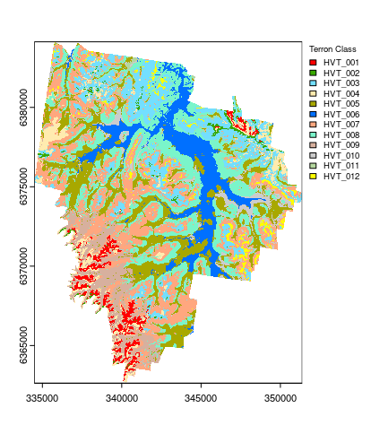
Apply model spatially
And finally the map that results from applying the hv.RF model to the covariate rasters.
## Apply model spatially class prediction
map.RF.c <- terra::predict(object = hv.rasters, model = hv.RF)

## plotting
map.RF.c <- as.factor(map.RF.c)

## HEX colors
area_colors <- c("#FF0000", "#38A800", "#73DFFF", "#FFEBAF", "#A8A800", "#0070FF", "#FFA77F", "#7AF5CA", "#D7B09E", "#CCCCCC", "#B4D79E", "#FFFF00")

terra::plot(map.RF.c, col = area_colors, plg = list(legend = c("HVT_001", "HVT_002", "HVT_003", "HVT_004", "HVT_005", "HVT_006", "HVT_007", "HVT_008", "HVT_009", "HVT_010", "HVT_011", "HVT_012"), cex = 0.75, title = "Terron Class"))
References
Malone, B P, P Hughes, A B McBratney, and B Minsany. 2014. “A Model for the Identification of Terrons in the Lower Hunter Valley, Australia.” Geoderma Regional 1: 31–47.