CODE:
Get the code used for this section here
Digital soil mapping using Random Forest algorithm
- Introduction
- Data preparation
- Perform the covariate intersection
- Model fitting
- Cross-validation
- Applying the model spatially
Introduction
A prevalent data mining algorithm in DSM and the soil sciences, and in applied sciences in general is the Random Forests algorithm. This algorithm is implemented in various forms across several different R packages. One of these, the randomForest package, can be used for both regression and classification purposes.
Random Forests are a boosted decision tree model. Further, Random Forests are an ensemble learning method for classification (and regression) that operate by constructing a multitude of decision trees at training time, which are later aggregated to give one single prediction for each observation in a data set.
For regression, the prediction is the average of the individual tree outputs, whereas in classification the trees vote by majority on the correct classification (mode). For further information regarding Random Forest and their underlying theory it is worth consulting Breiman (2001) and then Grimm et al. (2008) as an example of its application in DSM studies.
Data preparation
So lets firstly get the data organized. Recall from before in the data preparatory exercises that we were working with the soil point data and environmental covariates for the Hunter Valley area. These data are stored in the HV_subsoilpH object together with associated rasters supplied with the ithir package.
For the succession of models examined in these various pages, we will concentrate on modelling and mapping the soil pH for the 60-100cm depth interval. To refresh, lets load the data in, then intersect the data with the available covariates.
# libraries
library(ithir)
library(terra)
library(sf)
library(randomForest)

# point data
data(HV_subsoilpH)

# Start afresh round pH data to 2 decimal places
HV_subsoilpH$pH60_100cm <- round(HV_subsoilpH$pH60_100cm, 2)

# remove already intersected data
HV_subsoilpH <- HV_subsoilpH[, 1:3]

# add an id column
HV_subsoilpH$id <- seq(1, nrow(HV_subsoilpH), by = 1)

# re-arrange order of columns
HV_subsoilpH <- HV_subsoilpH[, c(4, 1, 2, 3)]

# Change names of coordinate columns
names(HV_subsoilpH)[2:3] <- c("x", "y")
# save a copy of coordinates
HV_subsoilpH$x2 <- HV_subsoilpH$x
HV_subsoilpH$y2 <- HV_subsoilpH$y

# convert data to sf object
HV_subsoilpH <- sf::st_as_sf(x = HV_subsoilpH, coords = c("x", "y"))

# grids (covariate rasters from ithir package)
hv.sub.rasters <- list.files(path = system.file("extdata/", package = "ithir"), pattern = "hunterCovariates_sub",
full.names = TRUE)

# read them into R as SpatRaster objects
hv.sub.rasters <- terra::rast(hv.sub.rasters)
Perform the covariate intersection
DSM_data <- terra::extract(x = hv.sub.rasters, y = HV_subsoilpH, bind = T, method = "simple")
DSM_data <- as.data.frame(DSM_data)
Often it is handy to check to see whether there are missing values both in the target variable and of the covariates. It is possible that a point location does not fit within the extent of the available covariates. In these cases the data should be excluded. A quick way to assess whether there are missing or NA values in the data is to use the complete.cases function.
which(!complete.cases(DSM_data))

## integer(0)

DSM_data <- DSM_data[complete.cases(DSM_data), ]
There do not appear to be any missing data as indicated by the integer(0) output above i.e there are zero rows with missing information.
Model fitting
Fitting a Random Forest model in R is relatively straightforward. It is worth consulting the the richly populated help files regarding the randomForest package and its functions. We will be using the randomForest function and a couple of extractor functions to tease out some of the model fitting diagnostics.
Familiar will be the formula structure of the model. As for the Cubist model, there are many model fitting parameters to consider such as the number of trees to build (ntree) and the number of variables (covariates) that are randomly sampled as candidates at each decision tree split (mtry), plus many others. The print function allows one to quickly assess the model fit. The importance parameter (logical variable) used within the randomForest function specifies that we want to also assess the importance of the covariates used.
Let’s have a look. First we perform the random subset to create the separate calibration and validation data sets.
set.seed(123)
training <- sample(nrow(DSM_data), 0.7 * nrow(DSM_data))
Now fit the model
hv.RF.Exp <- randomForest(pH60_100cm ~ AACN + Landsat_Band1 + Elevation + Hillshading +
Mid_Slope_Positon + MRVBF + NDVI + TWI, data = DSM_data[training, ], importance = TRUE,
ntree = 1000)

print(hv.RF.Exp)

##
## Call:
##  randomForest(formula = pH60_100cm ~ AACN + Landsat_Band1 + Elevation +      Hillshading + Mid_Slope_Positon + MRVBF + NDVI + TWI, data = DSM_data[training,      ], importance = TRUE, ntree = 1000)
##                Type of random forest: regression
##                      Number of trees: 1000
## No. of variables tried at each split: 2
##
##           Mean of squared residuals: 1.484758
##                     % Var explained: 15.33
Using the varImpPlot function allows one to visualize which covariates are of most importance to the prediction of our soil variable.
varImpPlot(hv.RF.Exp)
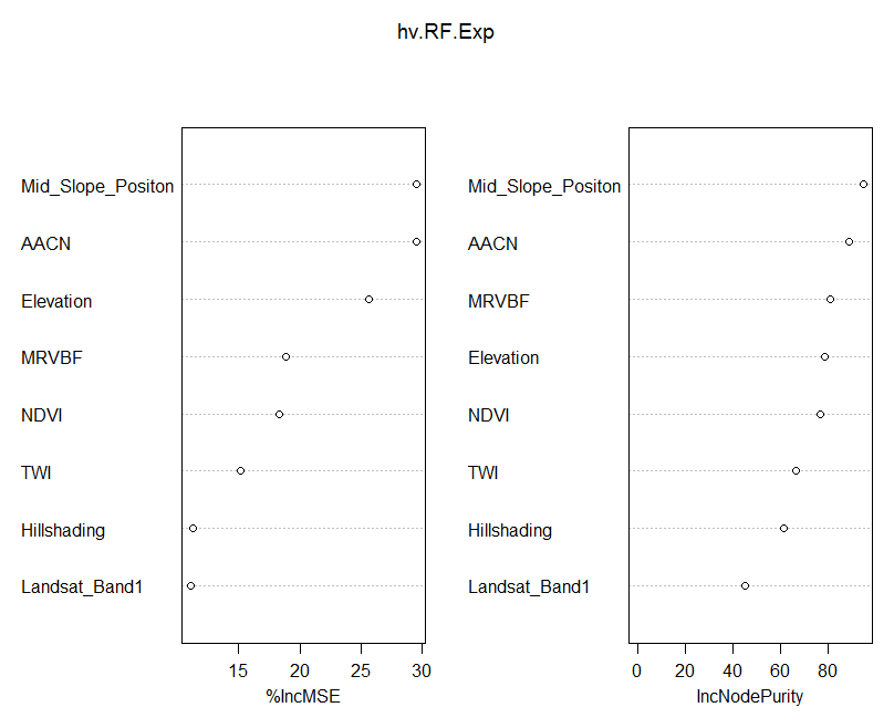
There is a lot of talk about how the variable importance is measured in Random Forest models. So it is probably best to quote from the source:
Here are the definitions of the variable importance measures. For each tree, the prediction accuracy on the out-of-bag portion of the data is recorded. Then the same is done after permuting each predictor variable. The difference between the two accuracy measurements are then averaged over all trees, and normalized by the standard error. For regression, the MSE is computed on the out-of-bag data for each tree, and then the same computed after permuting a variable. The differences are averaged and normalized by the standard error. If the standard error is equal to 0 for a variable, the division is not done (but the measure is almost always equal to 0 in that case). For the node purity, it is the total decrease in node impurities from splitting on the variable, averaged over all trees. For classification, the node impurity is measured by the Gini index. For regression, it is measured by residual sum of squares.
The important detail in the quotation above is the the variable importance is measured based on “out-of-bag”” samples. Which means observation not included in the model. Another detail is that they are based on an MSE accuracy measure; in this case the difference, when a covariate is included and excluded in a tree model. The value is averaged over all trees.
Cross-validation
So lets evaluate the hv.RF.Exp model both internally and externally.
# Internal validation
RF.pred.C <- predict(hv.RF.Exp, newdata = DSM_data[training, ])
goof(observed = DSM_data$pH60_100cm[training], predicted = RF.pred.C)

##          R2 concordance       MSE      RMSE         bias
## 1 0.9165725   0.8768092 0.3033557 0.5507774 0.0008385347

# External validation
RF.pred.V <- predict(hv.RF.Exp, newdata = DSM_data[-training, ])
goof(observed = DSM_data$pH60_100cm[-training], predicted = RF.pred.V)

##          R2 concordance     MSE     RMSE      bias
## 1 0.1856559   0.3090227 1.55794 1.248175 0.1013033
Essentially these results are quite similar to those of the validations from the other models. One needs to be careful about accepting very good model fit results without a proper external validation. This is particularly poignant for Random Forest models which have a tendency to provide excellent calibration results which can often give the wrong impression about its suitability for a given application. Therefore when using random forest models it pays to look at the validation on the out-of-bag samples when evaluating the goodness of fit of the model.
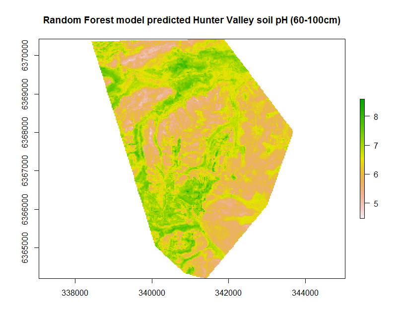
Apply model spatially
So lets look at the map resulting from applying the hv.RF.Exp models to the covariates.
## Apply model spatially
map.RF.r1 <- terra::predict(object = hv.sub.rasters, model = hv.RF.Exp, filename = "soilpH_60_100_RF.tif", datatype = "FLT4S", overwrite = TRUE)

plot(map.RF.r1, main = "Random Forest model predicted Hunter Valley soil pH (60-100cm)")
References
Breiman, L. 2001. “Random Forests.” Machine Learning 41: 5–32.
Grimm, R, T Behrens, M Marker, and H Elsenbeer. 2008. “Soil Organic Carbon Concentrations and Stocks on Barro Colorado Island: Digital Soil Mapping Using Random Forests Analysis.” Geoderma 146: 102–13.