CODE:
Get the code used for this section here
Hybrid Regression Kriging
- Introduction
- Data preparation
- Perform the covariate intersection
- Model fitting
- Out-of-bag model evaluation
- Spatial prediction
Introduction
The following example will provide the steps one might use to perform regression kriging that incorporates a complex model structure such as a data mining algorithm.
Here we will use the Cubist model that was also used earlier. Lets start from the top.
Data preparation
So lets firstly get the data organized. Recall from before in the data preparatory exercises that we were working with the soil point data and environmental covariates for the Hunter Valley area. These data are stored in the HV_subsoilpH object together with associated rasters supplied with the ithir package.
For the succession of models examined in these various pages, we will concentrate on modelling and mapping the soil pH for the 60-100cm depth interval. To refresh, lets load the data in, then intersect the data with the available covariates.
# libraries
library(ithir)
library(MASS)
library(terra)
library(sf)
library(gstat)
library(Cubist)

# point data
data(HV_subsoilpH)

# Start afresh round pH data to 2 decimal places
HV_subsoilpH$pH60_100cm <- round(HV_subsoilpH$pH60_100cm, 2)

# remove already intersected data
HV_subsoilpH <- HV_subsoilpH[, 1:3]

# add an id column
HV_subsoilpH$id <- seq(1, nrow(HV_subsoilpH), by = 1)

# re-arrange order of columns
HV_subsoilpH <- HV_subsoilpH[, c(4, 1, 2, 3)]

# Change names of coordinate columns
names(HV_subsoilpH)[2:3] <- c("x", "y")
# save a copy of coordinates
HV_subsoilpH$x2 <- HV_subsoilpH$x
HV_subsoilpH$y2 <- HV_subsoilpH$y

# convert data to sf object
HV_subsoilpH <- sf::st_as_sf(x = HV_subsoilpH, coords = c("x", "y"))

# grids (covariate rasters from ithir package)
hv.sub.rasters <- list.files(path = system.file("extdata/", package = "ithir"), pattern = "hunterCovariates_sub",
full.names = TRUE)

# read them into R as SpatRaster objects
hv.sub.rasters <- terra::rast(hv.sub.rasters)
Perform the covariate intersection
# extract covariate data
DSM_data <- terra::extract(x = hv.sub.rasters, y = HV_subsoilpH, bind = T, method = "simple")
DSM_data <- as.data.frame(DSM_data)
Often it is handy to check to see whether there are missing values both in the target variable and of the covariates. It is possible that a point location does not fit within the extent of the available covariates. In these cases the data should be excluded. A quick way to assess whether there are missing or NA values in the data is to use the complete.cases function.
which(!complete.cases(DSM_data))

## integer(0)

DSM_data <- DSM_data[complete.cases(DSM_data), ]
There do not appear to be any missing data as indicated by the integer(0) output above i.e there are zero rows with missing information.
Model Fitting
For the structural part of the regression kriging model, the cubist model algorithm is used and is effectively the same as what was covered here).
## Cubist modeling of environmental trend
set.seed(875)
training <- sample(nrow(DSM_data), 0.7 * nrow(DSM_data))
mDat <- DSM_data[training, ]
names(mDat)[3:4] <- c("x", "y")

# fit the model
hv.cub.Exp <- cubist(x = mDat[, c("AACN", "Landsat_Band1", "Elevation", "Hillshading", "Mid_Slope_Positon", "MRVBF", "NDVI", "TWI")], y = mDat$pH60_100cm, cubistControl(rules = 100, extrapolation = 15), committees = 1)
Now derive the model residual which is the model prediction subtracted from the residual.
## Model residuals
mDat$residual <- mDat$pH60_100cm - predict(hv.cub.Exp, newdata = mDat)
mean(mDat$residual)

## [1] 0.1086524

hist(mDat$residual)
If you check the histogram of these residuals you will find that the mean is around zero and the data seems normally distributed. Now we can assess the residuals for any spatial structure using a variogram model.
## calculate variogram
vgm1 <- variogram(residual ~ 1, ~x + y, mDat, width = 200, cutoff = 3000)

# initialise variogram model
mod <- vgm(psill = var(mDat$residual), "Sph", range = 3000, nugget = 0)

# fit model
model_1 <- fit.variogram(vgm1, mod)
model_1

##   model     psill    range
## 1   Nug 0.8030644    0.000
## 2   Sph 0.5676551 1111.159

plot(vgm1, model = model_1)

# Residual kriging model
gRK <- gstat(NULL, "RKresidual", residual ~ 1, locations = ~x + y, mDat, model = model_1)
Out-of-bag model evaluation
With the two model components together, we can now compare the model evaluations of using the Cubist model only to the hybrid estimate based on Cubist model predictions together with modeled residuals.
## Model evaluation on out-of-bag data Cubist model predictions
Cubist.pred.V <- predict(hv.cub.Exp, newdata = DSM_data[-training, ])

# Cubist model with residual variogram
vDat <- DSM_data[-training, ]
names(vDat)[3:4] <- c("x", "y")

# make the residual predictions
RK.preds.V <- krige(residual ~ 1, mDat, locations = ~x + y, model = model_1, newdata = vDat)

# Sum the two components together
RK.preds.fin <- Cubist.pred.V + RK.preds.V[, 3]

# evaluation based on cubist model only
goof(observed = DSM_data$pH60_100cm[-training], predicted = Cubist.pred.V, plot.it = T)

##          R2 concordance      MSE     RMSE        bias
## 1 0.1978859     0.33224 1.506298 1.227313 -0.05218972

# validation regression kriging with cubist model
goof(observed = DSM_data$pH60_100cm[-training], predicted = RK.preds.fin, plot.it = T)

##          R2 concordance      MSE     RMSE       bias
## 1 0.3372345   0.5236584 1.258334 1.121755 0.09227384
These results confirm that there to be some advantage in performing regression kriging with these soil data.
Spatial prediction
To apply the regression kriging model spatially, there are 3 basic steps.
- First apply the Cubist model,
- Then apply the residual kriging,
- Then finally add both maps together.
The script below illustrates how this is done.
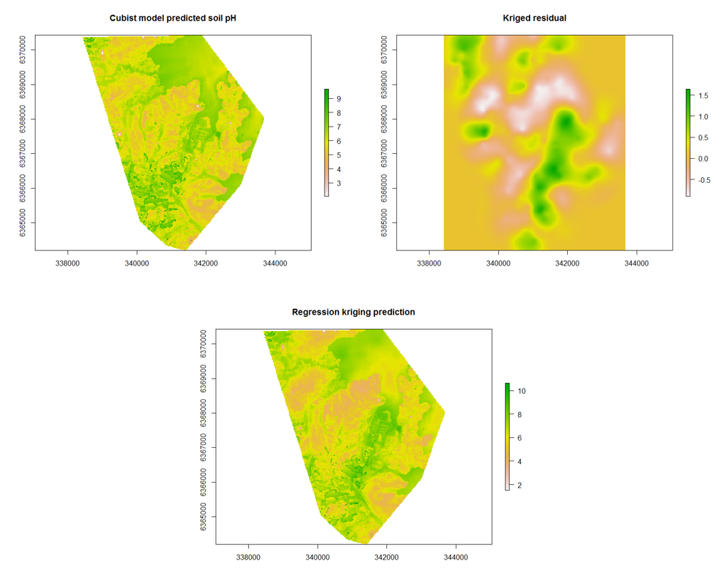
## Spatial prediction
par(mfrow = c(3, 1))

# Cubist model
map.RK1 <- terra::predict(object = hv.sub.rasters, model = hv.cub.Exp, filename = "soilpH_60_100_cubistRK.tif", datatype = "FLT4S", overwrite = TRUE)
plot(map.RK1, main = "Cubist model predicted soil pH")

## Interpolated residuals (note index of 1..get prediction only)
map.RK2 <- terra::interpolate(object = hv.sub.rasters, model = gRK, xyOnly = TRUE, index = 1, filename = "soilpH_60_100_residualRK.tif", datatype = "FLT4S", overwrite = TRUE)
plot(map.RK2, main = "Kriged residual")

## Sum of cubist predictions and residuals #Stack prediction and kriged
## residuals
pred.stack <- c(map.RK1, map.RK2)
map.RK3 <- sum(pred.stack)
plot(map.RK3, main = "Regression kriging prediction")