CODE:
Get the code used for this section here
Digital soil mapping using Decision Tree algorithm
- Introduction
- Data preparation
- Perform the covariate intersection
- Model fitting
- Cross-validation
- Applying the model spatially
Introduction
Linear regression is a global model, where there is a single predictive formula holding over the entire data space. With a linear model we therefore make some assumptions about how our target variable relates to the covariates.
These may often hold. However, it is models that allow one the flexibility of modelling non-linearity that are increasingly popular in the DSM community. One of these model structures are classification and regression trees (CART).
These models are a non-parametric decision tree learning algorithm that produces either classification or regression trees.
In this page we will concentrate on regression trees because our target variable is numeric i.e. a continuous variable. On another page we will look at classification trees for categorical variables. Decision trees (either regression or classification) are formed by a collection of rules based on variables in the modeling data set:
-
Rules based on variables’ values are selected to get the best split to differentiate observations based on the dependent variable.
-
Once a rule is selected and splits a node into two, the same process is applied to each subsequent node (i.e. it is a recursive procedure).
-
Splitting stops when CART detects no further gain can be made, or some pre-set stopping rules are met. Alternatively, the data are split as much as possible and then the tree is later pruned.
Each branch of the tree ends in a terminal node. Each observation falls into one and exactly one terminal node, and each terminal node is uniquely defined by a set of rules.
For a regression tree, the terminal node is a single value, or could be a regression model (which is the case for Cubist models which we will look at later).
Implementation of regression trees in R is provided both through the rpart and party packages. We will use the rpart package and its rpart function. However, the party package through the ctree function offers more functionality, and implements the partitioning in a more statistical robust fashion. Both functions however can handle both continuous and categorical predictor variables.
Data preparation
So lets firstly get the data organized. Recall from before in the data preparatory exercises that we were working with the soil point data and environmental covariates for the Hunter Valley area. These data are stored in the HV_subsoilpH object together with associated rasters supplied with the ithir package.
For the succession of models examined in these various pages, we will concentrate on modelling and mapping the soil pH for the 60-100cm depth interval. To refresh, lets load the data in, then intersect the data with the available covariates.
# libraries
library(ithir)
library(terra)
library(sf)
library(rpart)

# point data
data(HV_subsoilpH)

# Start afresh round pH data to 2 decimal places
HV_subsoilpH$pH60_100cm <- round(HV_subsoilpH$pH60_100cm, 2)

# remove already intersected data
HV_subsoilpH <- HV_subsoilpH[, 1:3]

# add an id column
HV_subsoilpH$id <- seq(1, nrow(HV_subsoilpH), by = 1)

# re-arrange order of columns
HV_subsoilpH <- HV_subsoilpH[, c(4, 1, 2, 3)]

# Change names of coordinate columns
names(HV_subsoilpH)[2:3] <- c("x", "y")
# save a copy of coordinates
HV_subsoilpH$x2 <- HV_subsoilpH$x
HV_subsoilpH$y2 <- HV_subsoilpH$y

# convert data to sf object
HV_subsoilpH <- sf::st_as_sf(x = HV_subsoilpH, coords = c("x", "y"))

# grids (covariate rasters from ithir package)
hv.sub.rasters <- list.files(path = system.file("extdata/", package = "ithir"), pattern = "hunterCovariates_sub", full.names = TRUE)

# read them into R as SpatRaster objects
hv.sub.rasters <- terra::rast(hv.sub.rasters)
Perform the covariate intersection
DSM_data <- terra::extract(x = hv.sub.rasters, y = HV_subsoilpH, bind = T, method = "simple")
DSM_data <- as.data.frame(DSM_data)
Often it is handy to check to see whether there are missing values both in the target variable and of the covariates. It is possible that a point location does not fit within the extent of the available covariates. In these cases the data should be excluded. A quick way to assess whether there are missing or NA values in the data is to use the complete.cases function.
# check for NA values
which(!complete.cases(DSM_data))

## integer(0)

DSM_data <- DSM_data[complete.cases(DSM_data), ]
There do not appear to be any missing data as indicated by the integer(0) output above i.e there are zero rows with missing information.
Model fitting
Fitting a decision tree in R is quite similar to that for linear models. Note that below we are also performing a random hold-back of some data for an external validation.
## Fitting a decision tree model
set.seed(123)
training <- sample(nrow(DSM_data), 0.7 * nrow(DSM_data))

hv.RT.Exp <- rpart(pH60_100cm ~ AACN + Landsat_Band1 + Elevation + Hillshading +
Mid_Slope_Positon + MRVBF + NDVI + TWI, data = DSM_data[training, ], control = rpart.control(minsplit = 50))
It is worthwhile to look at the help file for rpart particularly those aspects regarding the rpart.control parameters which control the rpart fit. Often it is helpful to just play around with the parameters to get a sense of what does what. Here for the minsplit parameter within rpart.control we are specifying that we want at least 50 observations in a node in order for a split to be attempted.
Detailed results of the model fit can be provided via the summary and printcp functions.
summary(hv.RT.Exp)

## Call:
## rpart(formula = pH60_100cm ~ AACN + Landsat_Band1 + Elevation +
##     Hillshading + Mid_Slope_Positon + MRVBF + NDVI + TWI, data = DSM_data[training,
##     ], control = rpart.control(minsplit = 50))
##   n= 354
##
##           CP nsplit rel error    xerror       xstd
## 1 0.06794766      0 1.0000000 1.0050406 0.06360731
## 2 0.03317748      2 0.8641047 1.0228037 0.06761617
## 3 0.03220587      3 0.8309272 0.9935433 0.06698589
## 4 0.02195220      6 0.7343096 0.9645777 0.06626158
## 5 0.02155232      7 0.7123574 0.9680294 0.07002215
## 6 0.01287867      8 0.6908051 0.9768363 0.07142329
## 7 0.01234328      9 0.6779264 0.9753883 0.07151362
## 8 0.01000000     10 0.6655831 0.9754643 0.07164849
##
## Variable importance
##              AACN               TWI         Elevation             MRVBF
##                22                18                14                13
## Mid_Slope_Positon              NDVI       Hillshading     Landsat_Band1
##                11                10                 9                 4
##
## Node number 1: 354 observations,    complexity param=0.06794766
##   mean=6.55096, MSE=1.753635
##   left son=2 (272 obs) right son=3 (82 obs)
##   Primary splits:
##       AACN              < 43.59965   to the left,  improve=0.06379266, (0 missing)
##       Mid_Slope_Positon < 0.783947   to the left,  improve=0.06097348, (0 missing)
##       MRVBF             < 0.0166785  to the right, improve=0.05881503, (0 missing)
##       TWI               < 9.806141   to the right, improve=0.05306808, (0 missing)
##       Elevation         < 182.9988   to the left,  improve=0.03736796, (0 missing)
##   Surrogate splits:
##       Elevation         < 154.1056   to the left,  agree=0.958, adj=0.817, (0 split)
##       TWI               < 9.704844   to the right, agree=0.915, adj=0.634, (0 split)
##       MRVBF             < 0.025861   to the right, agree=0.879, adj=0.476, (0 split)
##       Hillshading       < 14.0666    to the left,  agree=0.802, adj=0.146, (0 split)
##       Mid_Slope_Positon < 0.011807   to the right, agree=0.771, adj=0.012, (0 split)
##
## Node number 2: 272 observations,    complexity param=0.06794766
##   mean=6.367316, MSE=1.691953
##   left son=4 (179 obs) right son=5 (93 obs)
##   Primary splits:
##       Mid_Slope_Positon < 0.7870535  to the left,  improve=0.09726051, (0 missing)
##       MRVBF             < 0.62053    to the left,  improve=0.08383424, (0 missing)
##       TWI               < 17.16774   to the left,  improve=0.07594164, (0 missing)
##       AACN              < 3.510582   to the right, improve=0.06521629, (0 missing)
##       Elevation         < 99.58687   to the right, improve=0.05214677, (0 missing)
##   Surrogate splits:
##       TWI         < 16.32056   to the left,  agree=0.897, adj=0.699, (0 split)
##       AACN        < 6.921867   to the right, agree=0.868, adj=0.613, (0 split)
##       MRVBF       < 1.858052   to the left,  agree=0.860, adj=0.591, (0 split)
##       Hillshading < 2.116992   to the right, agree=0.794, adj=0.398, (0 split)
##       Elevation   < 101.4914   to the right, agree=0.746, adj=0.258, (0 split)
##
## Node number 3: 82 observations,    complexity param=0.02155232
##   mean=7.160122, MSE=1.475291
##   left son=6 (26 obs) right son=7 (56 obs)
##   Primary splits:
##       NDVI        < -0.2270705 to the left,  improve=0.11059740, (0 missing)
##       MRVBF       < 0.0181425  to the right, improve=0.10021720, (0 missing)
##       Hillshading < 7.197221   to the left,  improve=0.07748013, (0 missing)
##       Elevation   < 161.3855   to the right, improve=0.06811931, (0 missing)
##       AACN        < 75.9357    to the left,  improve=0.06218024, (0 missing)
##   Surrogate splits:
##       Landsat_Band1     < 42.5       to the left,  agree=0.793, adj=0.346, (0 split)
##       Mid_Slope_Positon < 0.1866335  to the left,  agree=0.744, adj=0.192, (0 split)
##       Hillshading       < 11.70925   to the right, agree=0.720, adj=0.115, (0 split)
##       MRVBF             < 0.303978   to the right, agree=0.695, adj=0.038, (0 split)
##       TWI               < 10.23516   to the right, agree=0.695, adj=0.038, (0 split)
##
## Node number 4: 179 observations,    complexity param=0.03317748
##   mean=6.074916, MSE=1.625561
##   left son=8 (34 obs) right son=9 (145 obs)
##   Primary splits:
##       AACN          < 13.55327   to the left,  improve=0.07078306, (0 missing)
##       NDVI          < -0.1660675 to the left,  improve=0.04227382, (0 missing)
##       Hillshading   < 3.38458    to the left,  improve=0.03978021, (0 missing)
##       Landsat_Band1 < 52.5       to the right, improve=0.03485309, (0 missing)
##       TWI           < 15.09922   to the right, improve=0.02528861, (0 missing)
##   Surrogate splits:
##       TWI               < 14.49579   to the right, agree=0.888, adj=0.412, (0 split)
##       Elevation         < 101.5807   to the left,  agree=0.849, adj=0.206, (0 split)
##       MRVBF             < 2.628778   to the right, agree=0.849, adj=0.206, (0 split)
##       Mid_Slope_Positon < 0.7812145  to the right, agree=0.821, adj=0.059, (0 split)
##       Hillshading       < 0.9076225  to the left,  agree=0.816, adj=0.029, (0 split)
##
## Node number 5: 93 observations,    complexity param=0.01234328
##   mean=6.930108, MSE=1.338444
##   left son=10 (73 obs) right son=11 (20 obs)
##   Primary splits:
##       NDVI      < -0.1538785 to the left,  improve=0.06155876, (0 missing)
##       MRVBF     < 2.748072   to the left,  improve=0.04850123, (0 missing)
##       Elevation < 99.90028   to the right, improve=0.03367224, (0 missing)
##       TWI       < 16.79354   to the left,  improve=0.03088351, (0 missing)
##       AACN      < 3.648288   to the right, improve=0.02936984, (0 missing)
##   Surrogate splits:
##       Landsat_Band1 < 63.5       to the left,  agree=0.796, adj=0.05, (0 split)
##
## Node number 6: 26 observations
##   mean=6.567308, MSE=1.515658
##
## Node number 7: 56 observations,    complexity param=0.01287867
##   mean=7.435357, MSE=1.217632
##   left son=14 (37 obs) right son=15 (19 obs)
##   Primary splits:
##       Elevation     < 165.3835   to the right, improve=0.11724900, (0 missing)
##       TWI           < 9.119365   to the left,  improve=0.06946874, (0 missing)
##       MRVBF         < 0.016642   to the right, improve=0.05460568, (0 missing)
##       AACN          < 59.41751   to the right, improve=0.04961327, (0 missing)
##       Landsat_Band1 < 51         to the right, improve=0.03827830, (0 missing)
##   Surrogate splits:
##       AACN        < 59.41751   to the right, agree=0.946, adj=0.842, (0 split)
##       TWI         < 9.690168   to the left,  agree=0.768, adj=0.316, (0 split)
##       Hillshading < 3.093062   to the right, agree=0.750, adj=0.263, (0 split)
##       MRVBF       < 0.145624   to the left,  agree=0.732, adj=0.211, (0 split)
##       NDVI        < -0.1460055 to the left,  agree=0.714, adj=0.158, (0 split)
##
## Node number 8: 34 observations
##   mean=5.374412, MSE=1.01446
##
## Node number 9: 145 observations,    complexity param=0.03220587
##   mean=6.239172, MSE=1.626812
##   left son=18 (120 obs) right son=19 (25 obs)
##   Primary splits:
##       TWI       < 13.928     to the left,  improve=0.07823863, (0 missing)
##       MRVBF     < 0.62053    to the left,  improve=0.06765783, (0 missing)
##       NDVI      < -0.161967  to the left,  improve=0.04928153, (0 missing)
##       Elevation < 142.9022   to the right, improve=0.03381342, (0 missing)
##       AACN      < 21.32139   to the right, improve=0.02651395, (0 missing)
##   Surrogate splits:
##       AACN        < 17.50792   to the right, agree=0.883, adj=0.32, (0 split)
##       MRVBF       < 1.790583   to the left,  agree=0.876, adj=0.28, (0 split)
##       Elevation   < 107.4445   to the right, agree=0.855, adj=0.16, (0 split)
##       Hillshading < 2.147379   to the right, agree=0.834, adj=0.04, (0 split)
##
## Node number 10: 73 observations
##   mean=6.779863, MSE=1.317859
##
## Node number 11: 20 observations
##   mean=7.4785, MSE=1.030453
##
## Node number 14: 37 observations
##   mean=7.164595, MSE=1.108441
##
## Node number 15: 19 observations
##   mean=7.962632, MSE=1.009483
##
## Node number 18: 120 observations,    complexity param=0.03220587
##   mean=6.076333, MSE=1.468697
##   left son=36 (47 obs) right son=37 (73 obs)
##   Primary splits:
##       Landsat_Band1 < 52.5       to the right, improve=0.09342719, (0 missing)
##       NDVI          < -0.1709515 to the left,  improve=0.06335787, (0 missing)
##       Hillshading   < 3.976624   to the left,  improve=0.05009109, (0 missing)
##       MRVBF         < 0.629809   to the left,  improve=0.04625149, (0 missing)
##       AACN          < 29.02258   to the left,  improve=0.04051094, (0 missing)
##   Surrogate splits:
##       NDVI        < -0.2207    to the right, agree=0.675, adj=0.170, (0 split)
##       AACN        < 18.27993   to the left,  agree=0.658, adj=0.128, (0 split)
##       Elevation   < 104.9371   to the left,  agree=0.642, adj=0.085, (0 split)
##       MRVBF       < 0.0307535  to the left,  agree=0.642, adj=0.085, (0 split)
##       Hillshading < 9.895688   to the right, agree=0.625, adj=0.043, (0 split)
##
## Node number 19: 25 observations
##   mean=7.0208, MSE=1.647543
##
## Node number 36: 47 observations
##   mean=5.614681, MSE=0.744344
##
## Node number 37: 73 observations,    complexity param=0.03220587
##   mean=6.373562, MSE=1.7095
##   left son=74 (50 obs) right son=75 (23 obs)
##   Primary splits:
##       NDVI              < -0.176242  to the left,  improve=0.20079140, (0 missing)
##       Hillshading       < 3.976624   to the left,  improve=0.13627740, (0 missing)
##       MRVBF             < 0.6187865  to the left,  improve=0.03184879, (0 missing)
##       Mid_Slope_Positon < 0.6320945  to the right, improve=0.02794618, (0 missing)
##       Elevation         < 142.8409   to the right, improve=0.01737568, (0 missing)
##   Surrogate splits:
##       Elevation < 117.1724   to the right, agree=0.699, adj=0.043, (0 split)
##
## Node number 74: 50 observations,    complexity param=0.0219522
##   mean=5.9762, MSE=1.051936
##   left son=148 (26 obs) right son=149 (24 obs)
##   Primary splits:
##       Hillshading   < 5.843943   to the left,  improve=0.25909640, (0 missing)
##       Landsat_Band1 < 47.5       to the left,  improve=0.11351230, (0 missing)
##       AACN          < 29.47343   to the left,  improve=0.10966650, (0 missing)
##       MRVBF         < 0.478392   to the left,  improve=0.10308040, (0 missing)
##       NDVI          < -0.295995  to the left,  improve=0.08545253, (0 missing)
##   Surrogate splits:
##       Elevation         < 128.4046   to the left,  agree=0.72, adj=0.417, (0 split)
##       TWI               < 9.897047   to the right, agree=0.68, adj=0.333, (0 split)
##       AACN              < 33.61438   to the left,  agree=0.66, adj=0.292, (0 split)
##       MRVBF             < 0.0682475  to the right, agree=0.64, adj=0.250, (0 split)
##       Mid_Slope_Positon < 0.6506405  to the right, agree=0.62, adj=0.208, (0 split)
##
## Node number 75: 23 observations
##   mean=7.237391, MSE=2.049532
##
## Node number 148: 26 observations
##   mean=5.474615, MSE=0.2419556
##
## Node number 149: 24 observations
##   mean=6.519583, MSE=1.361596
The summary output provides detailed information of the data splitting as well as information as to the relative importance of the covariates.
printcp(hv.RT.Exp)

##
## Regression tree:
## rpart(formula = pH60_100cm ~ AACN + Landsat_Band1 + Elevation +
##     Hillshading + Mid_Slope_Positon + MRVBF + NDVI + TWI, data = DSM_data[training,
##     ], control = rpart.control(minsplit = 50))
##
## Variables actually used in tree construction:
## [1] AACN              Elevation         Hillshading       Landsat_Band1
## [5] Mid_Slope_Positon NDVI              TWI
##
## Root node error: 620.79/354 = 1.7536
##
## n= 354
##
##         CP nsplit rel error  xerror     xstd
## 1 0.067948      0   1.00000 1.00504 0.063607
## 2 0.033177      2   0.86410 1.02280 0.067616
## 3 0.032206      3   0.83093 0.99354 0.066986
## 4 0.021952      6   0.73431 0.96458 0.066262
## 5 0.021552      7   0.71236 0.96803 0.070022
## 6 0.012879      8   0.69081 0.97684 0.071423
## 7 0.012343      9   0.67793 0.97539 0.071514
## 8 0.010000     10   0.66558 0.97546 0.071648
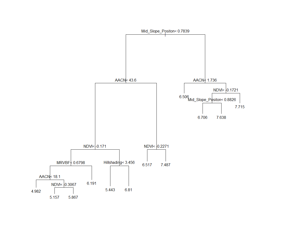
The printcp function provides the useful output of indicating which covariates were included in the final model. For the visually inclined, a plot of the tree assists a lot to interpret the model diagnostics and assessing the important covariates too.
plot(hv.RT.Exp)
text(hv.RT.Exp)
Cross-validation
As before, we can use the goof function to evaluate the performance of the model fit both internally and externally.
## Goodness of fit evaluation
# Internal validation
RT.pred.C <- predict(hv.RT.Exp, DSM_data[training, ])
goof(observed = DSM_data$pH60_100cm[training], predicted = RT.pred.C)

##          R2 concordance     MSE     RMSE bias
## 1 0.3344169   0.4998021 1.16719 1.080366    0

# External validation
RT.pred.V <- predict(hv.RT.Exp, DSM_data[-training, ])
goof(observed = DSM_data$pH60_100cm[-training], predicted = RT.pred.V)

##          R2 concordance      MSE    RMSE       bias
## 1 0.1537061   0.3426565 1.690599 1.30023 0.04590521
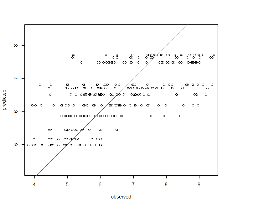
The decision tree model performance is not too dissimilar to the MLR model. Looking at the xy-plot from the external validation above and the decision tree, it becomes clear that a potential issue is apparent. This is, there are only a finite number of possible outcomes in terms of the predictions.
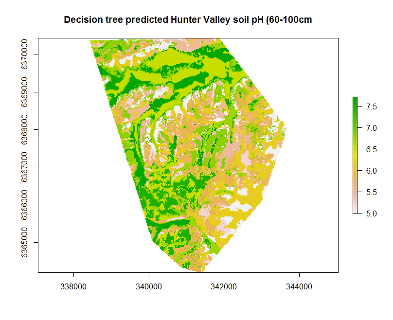
Spatial prediction
This finite property becomes obviously apparent once we make a map by applying the fitted model to the covariates (using the terra::predict function and hv.sub.rasters object).
## Create the map
map.RT.r1 <- terra::predict(object = hv.sub.rasters, model = hv.RT.Exp, filename = "soilpH_60_100_RT.tif", datatype = "FLT4S", overwrite = TRUE)

plot(map.RT.r1, main = "Decision tree predicted Hunter Valley soil pH (60-100cm")