CODE:
Get the code used for this section here
Bootstrapping for uncertainty estimation
- Pre-work reading
- Defining the model parameters
- Mapping predictions and model uncertainties
- Evaluating the quantification of uncertainties
Pre-work reading
Bootstrapping is a non-parametric approach for quantifying prediction uncertainties (Efron and Tibshirani 1993). Bootstrapping involves repeated random sampling with replacement of the available data. With the bootstrap sample, a model is fitted, and can then be applied to generate a digital soil map. By repeating the process of random sampling and applying the model, we are able to generate probability distributions of the prediction realizations from each model at each pixel.
A robust estimate may be determined by taking the average of all the simulated predictions at each pixel. By being able to obtain probability distributions of the outcomes, one is also able to quantify the uncertainty of the modeling by computing a prediction interval given a specified level of confidence.
While the bootstrapping approach is relatively straightforward, it can be computationally expensive as more robust estimations are expected as the number of iterations increases. This obviously could be prohibitive from a computational and data storage point of view, but not altogether impossible (given parallel processing capabilities etc.) as was demonstrated by both Malone and Searle (2021) and Liddicoat et al. (2015) whom both performed bootstrapping for quantification of uncertainties across very large mapping extents. In the case of Malone and Searle (2021) this for for the entire Australian continent at 100m resolution.
In the example below, the bootstrap method is demonstrated. We will be using Cubist modeling for the model structure and perform 50 bootstrap iterations. We will do the bootstrap model using 70% of the available data. The remaining 30% will be used for an out-of-bag model evaluation and therefore separated entirely from any model calibration function.
Defining the model parameters
For the first step, we do the random partitioning of the data into calibration and validation data sets. Again we are using the HV_subsoilpH data from the ithir package and the associated covariates that come shipped with the package
# Libraries
library(ithir)
library(sf)
library(terra)
library(Cubist)

# point data
data(HV_subsoilpH)

# Start afresh round pH data to 2 decimal places
HV_subsoilpH$pH60_100cm <- round(HV_subsoilpH$pH60_100cm, 2)

# remove already intersected data
HV_subsoilpH <- HV_subsoilpH[, 1:3]

# add an id column
HV_subsoilpH$id <- seq(1, nrow(HV_subsoilpH), by = 1)

# re-arrange order of columns
HV_subsoilpH <- HV_subsoilpH[, c(4, 1, 2, 3)]

# Change names of coordinate columns
names(HV_subsoilpH)[2:3] <- c("x", "y")
# save a copy of coordinates
HV_subsoilpH$x2 <- HV_subsoilpH$x
HV_subsoilpH$y2 <- HV_subsoilpH$y

# convert data to sf object
HV_subsoilpH <- sf::st_as_sf(x = HV_subsoilpH, coords = c("x", "y"))

# grids (covariate rasters from ithir package)
hv.sub.rasters <- list.files(path = system.file("extdata/", package = "ithir"), pattern = "hunterCovariates_sub", full.names = TRUE)

# read them into R as SpatRaster objects
hv.sub.rasters <- terra::rast(hv.sub.rasters)

# extract covariate data
DSM_data <- terra::extract(x = hv.sub.rasters, y = HV_subsoilpH, bind = T, method = "simple")
DSM_data <- as.data.frame(DSM_data)

# check for NA values
which(!complete.cases(DSM_data))

## integer(0)

DSM_data <- DSM_data[complete.cases(DSM_data), ]

# subset data for modeling
set.seed(123)
training <- sample(nrow(DSM_data), 0.7 * nrow(DSM_data))
DSM_data_cal <- DSM_data[training, ]  # calibration
DSM_data_val <- DSM_data[-training, ]  # validation

# Number of bootstrap iterations
nbag <- 50
The nbag variable below holds the value for the number of bootstrap models we want to fit. Here it is 50.
Essentially the bootstrap can can be contained within a for loop, where upon each loop a sample of the available data is taken of n size where the n is the same number of cases in the model frame. This sampling is done with replacement, which works out to be about 66% of the data in terms of unique cases. The other 34% of the data could be used to assess the model goodness of fit for each bootstrap iteration in terms of out-of-bag assessment, which just means data not included in the model. Note that this particular out-of-bag assessment if different to the one we use in this example which is based on the random hold strategy and was implemented right at the beginning. None of these data cases will be exposed to a model fitting situation, but in the cases of the bootstrapping some cases will be used for both calibration and out-of-bag evaluation depending on the modeling iteration.
Note below the use of the replace parameter to indicate we want a random sample with replacement. After a model is fitted, we save the model to file and will come back to it later. The modelFile variable shows the extensive use of the paste0 function in order to provide the pathway and file name for the model that we want to save on each loop iteration.
The saveRDS function allows us to save each of the model objects as rds files to the location specified. An alternative to save the models individually to file is to save them to elements within a list. When dealing with very large numbers of models and additionally are complex in terms of their parameterizations, the save to list elements alternative could run into computer memory limitation issues. The last section of the script below just demonstrates the use of the list.files functions to confirm that we have saved those models to file and they are ready to use.
# Fit cubist models for each bootstrap
for (i in 1:nbag) {
  # sample with replacement
  sample.wr <- sample.int(n = nrow(DSM_data_cal), size = nrow(DSM_data_cal), replace = TRUE)
  # unique cases
  sample.wr <- unique(sample.wr)
  # fit model
  fit_cubist <- cubist(x = DSM_data_cal[sample.wr, 5:15], y = DSM_data_cal$pH60_100cm[sample.wr], cubistControl(rules = 5, extrapolation = 5), committees = 1)

  ### Note you will likely have different file path names ###
  modelFile <- paste0("bootMod_", i, ".rds")
  saveRDS(object = fit_cubist, file = modelFile)}
We can then assess the model goodness of fit of each bootstrap, or collectively in summary.. This is done using the goof function as in previous examples. This time we incorporate that function within a for loop. For each loop, we read in the model via the radRDS function and then save the diagnostics to the cubiMat.cal or cubiMat.val matrix objects depending on whether the calibration or out-of-bag sample data cases.
After the iterations are completed, we use the colMeans function to calculate the means of the diagnostics over the 50 model iterations. You could also assess the variance of those means by a command such as var(cubiDat.val[,1]), which would return the variance of the R2 values. Similarly you could plot a histogram of one of the metrics to get a visual sense of how different data configurations result in slightly to major different model evaluations. Ideally you would not want a large spread of these results, but some dispersion should be expected as each fitted model see different configurations of the data on each iteration.
# list all model files in directory Note you will likely have different file
# path names ###
c.models <- list.files(path = "SOME_DIRECTORY", pattern = "\\.rds$", full.names = TRUE)

head(c.models)

## [1] "~//bootMod_1.rds"
## [2] "~//bootMod_10.rds"
## [3] "~//bootMod_11.rds"
## [4] "~//bootMod_12.rds"
## [5] "~//bootMod_13.rds"
## [6] "~//bootMod_14.rds"

# model evaluation calibration data
cubiMat.cal <- matrix(NA, nrow = nbag, ncol = 5)
for (i in 1:nbag) {
  fit_cubist <- readRDS(c.models[i])
  cubiMat.cal[i, ] <- as.matrix(goof(observed = DSM_data_cal$pH60_100cm, predicted = predict(fit_cubist, newdata = DSM_data_cal)))}

cubiMat.cal <- as.data.frame(cubiMat.cal)
names(cubiMat.cal) <- c("R2", "concordance", "MSE", "RMSE", "bias")
colMeans(cubiMat.cal)

##          R2 concordance         MSE        RMSE        bias
##  0.22049885  0.37381139  1.38000709  1.17459380 -0.06808544

hist(cubiMat.cal$concordance)

# out-of-bag data
cubiMat.valpreds <- matrix(NA, ncol = nbag, nrow = nrow(DSM_data_val))
cubiMat.val <- matrix(NA, nrow = nbag, ncol = 5)
for (i in 1:nbag) {
  fit_cubist <- readRDS(c.models[i])
  cubiMat.valpreds[, i] <- predict(fit_cubist, newdata = DSM_data_val)
  cubiMat.val[i, ] <- as.matrix(goof(observed = DSM_data_val$pH60_100cm, predicted = predict(fit_cubist, newdata = DSM_data_val)))}

# mean predicted value
cubiMat.valpreds.MEAN <- rowMeans(cubiMat.valpreds)

cubiMat.val <- as.data.frame(cubiMat.val)
names(cubiMat.val) <- c("R2", "concordance", "MSE", "RMSE", "bias")
colMeans(cubiMat.val)

##           R2  concordance          MSE         RMSE         bias
##  0.213176496  0.358170500  1.507508458  1.227406694 -0.001465801

hist(cubiMat.val$concordance)

# Average out-of- bag MSE (systematic model error)
avGMSE <- mean(cubiMat.val[, 3])
avGMSE

## [1] 1.507508
For the out-of-bag cases, in addition to deriving the model diagnostic statistics, we are also saving the actual model predictions for these data for each iteration to the cubiMat.valpreds object. These will be used further on for evaluating the prediction uncertainties.
The last line of the script above saves the mean of the mean square error (MSE) estimates from the validation data. The independent MSE estimator, accounts for both systematic and random errors in the modeling. This estimate of the MSE is needed for quantifying the uncertainties, as this error is in addition to that which are accounted for by the bootstrap model, which are specifically those associated with the deterministic model component i.e. the model relationship between target variable and the covariates.
Subsequently an overall prediction variance (at each point or pixel) will be the sum of the random error component (MSE) and the bootstrap prediction variance (as estimated from the mean of the realisations from the bootstrap modeling).
Mapping predictions and model uncertainties
Our initial purpose here is to derive the mean and the variance of the predictions from each bootstrap sample. This requires loading in each bootstrap model, applying into the covariate data, then saving the predicted map to file or R memory. In the case below the predictions are saved to file. This is illustrated in the following script:
## Mapping ### Note you will likely have different file path names ###
for (i in 1:nbag) {
  fit_cubist <- readRDS(c.models[i])
  mapFile <- paste0("bootMap_", i, ".tif")
  # predict
  terra::predict(object = hv.sub.rasters, model = fit_cubist, filename = mapFile, overwrite = T)}
To evaluate the mean at each pixel from each of the created maps, the terra::app function is used which allows both existing and custom functions to be used to apply statistical analyses and summaries of raster data. The mean and var functions are examples of standard functions able to be incorporated into the terra::app functionality.
First we need to get the path location of the rasters. Notice from the list.files function and the pattern parameter, we are restricting the search of rasters that contain the string bootMap. Next we make a stack of those rasters, followed by the calculation of the mean and variance. As we can add variances and not standard deviations, the final prediction variance is simply the sum of the variance of bootstrap derived maps and the estimate of the systematic and random models (avGMSE) that was calculated earlier from the out-of-bag data cases.
## statistical measures of maps #Pathway to rasters ### Note you will likely
## have different file path names ###
map.files <- list.files(path = "SOME_DIRECTORY", pattern =  "bootMap", full.names = TRUE)
head(map.files)

# Raster stack all maps
pred.stack <- terra::rast(map.files)

# calculate mean
bootMap.mean <- terra::app(x = pred.stack, fun = mean)
# mask
msk <- terra::ifel(is.na(hv.sub.rasters[[1]]), NA, 1)
bootMap.mean <- terra::mask(bootMap.mean, msk, inverse = F)

# calculate variance
bootMap.var <- terra::app(x = pred.stack, fun = var)

# overall prediction variance (adding avGMSE)
bootMap.varF <- bootMap.var + avGMSE
To derive to 90% prediction interval we take the square root of the variance estimate and multiply that value by the quantile function value that corresponds to a 90% probability. The z value is obtained using the qnorm function. The standard error is then either added or subtracted to the mean prediction in order to generate the upper and lower prediction limits respectively.
# Standard deviation
bootMap.sd <- sqrt(bootMap.varF)

# standard error
bootMap.se <- bootMap.sd * qnorm(0.95)

# upper prediction limit
bootMap.upl <- bootMap.mean + bootMap.se
bootMap.upl <- terra::mask(bootMap.upl, msk, inverse = F)

# lower prediction limit
bootMap.lpl <- bootMap.mean - bootMap.se
bootMap.lpl <- terra::mask(bootMap.lpl, msk, inverse = F)

# prediction interval range
bootMap.pir <- bootMap.upl - bootMap.lpl
bootMap.pir <- terra::mask(bootMap.pir, msk, inverse = F)
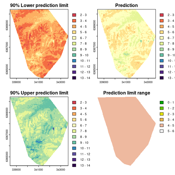
As for the Universal kriging example, we can plot the associated maps of the predictions and quantified uncertainties.
## PLOTTING
phCramp <- c("#d53e4f", "#f46d43", "#fdae61", "#fee08b", "#ffffbf", "#e6f598", "#abdda4", "#66c2a5", "#3288bd", "#5e4fa2", "#542788", "#2d004b")

brk <- c(2:14)
par(mfrow = c(2, 2))
plot(bootMap.lpl, main = "90% Lower prediction limit", breaks = brk, col = phCramp)
plot(bootMap.mean, main = "Prediction", breaks = brk, col = phCramp)
plot(bootMap.upl, main = "90% Upper prediction limit", breaks = brk, col = phCramp)
plot(bootMap.pir, main = "Prediction limit range", col = terrain.colors(length(seq(0, 6.5, by = 1)) - 1), axes = FALSE, breaks = seq(0, 6.5, by = 1))
Evaluating the quantification of uncertainties
You will recall the bootstrap model predictions on the validation data were saved to the cubiMat.valpreds object. We want estimate the standard deviation of those predictions for each point. Also recall that the prediction variance is the sum of the derivedavGMSE value (systematic model error) and the bootstrap sampling model prediction variance. Taking the square root of that summation results in standard deviation estimate.
## out-of-bag model evaluation
colMeans(cubiMat.val)

##           R2  concordance          MSE         RMSE         bias
##  0.213176496  0.358170500  1.507508458  1.227406694 -0.001465801

hist(cubiMat.val$concordance)

# calculate prediction standard deviation including systematic error
val.sd <- matrix(NA, ncol = 1, nrow = nrow(cubiMat.valpreds))
for (i in 1:nrow(cubiMat.valpreds)) {
  val.sd[i, 1] <- sqrt(var(cubiMat.valpreds[i, ]) + avGMSE)}
We then need to multiply the standard deviation by the corresponding percentile of the standard normal distribution in order to express the prediction limits at each level of confidence. Note the use of the for loop and the associated cycling through of the different percentile values.
# Percentiles of normal distribution
qp <- qnorm(c(0.995, 0.9875, 0.975, 0.95, 0.9, 0.8, 0.7, 0.6, 0.55, 0.525))

# z factor multiplication (standard error)
vMat <- matrix(NA, nrow = nrow(cubiMat.valpreds), ncol = length(qp))
for (i in 1:length(qp)) {
  vMat[, i] <- val.sd * qp[i]}
Now we add or subtract the limits from the averaged model predictions to derive to prediction limits for each case, for each level of confidence.
# upper prediction limit
uMat <- matrix(NA, nrow = nrow(cubiMat.valpreds), ncol = length(qp))
for (i in 1:length(qp)) {
  uMat[, i] <- cubiMat.valpreds.MEAN + vMat[, i]}

# lower prediction limit
lMat <- matrix(NA, nrow = nrow(cubiMat.valpreds), ncol = length(qp))
for (i in 1:length(qp)) {
  lMat[, i] <- cubiMat.valpreds.MEAN - vMat[, i]}
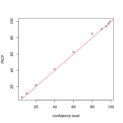
Now we assess the PICP for each level confidence. Recalling that we are simply assessing whether the observed value is encapsulated by the corresponding prediction limits, then calculating the proportion of agreement to total number of observations.
## PICP
bMat <- matrix(NA, nrow = nrow(cubiMat.valpreds), ncol = length(qp))
for (i in 1:ncol(bMat)) {
  bMat[, i] <- as.numeric(DSM_data_val$pH60_100cm <= uMat[, i] & DSM_data_val$pH60_100cm >= lMat[, i])}

# make plot
par(mfrow = c(1, 1))
cs <- c(99, 97.5, 95, 90, 80, 60, 40, 20, 10, 5)
plot(cs, ((colSums(bMat)/nrow(bMat)) * 100), ylab = "PICP", xlab = "confidence level")
# draw 1:1 line
abline(a = 0, b = 1, col = "red")

## Prediction limit range 90% PI
cs <- c(99, 97.5, 95, 90, 80, 60, 40, 20, 10, 5)
colnames(lMat) <- cs
colnames(uMat) <- cs
quantile(uMat[, "90"] - lMat[, "90"])

##       0%      25%      50%      75%     100%
## 4.060951 4.092680 4.112038 4.144268 4.367537
References
Efron, B., and R. Tibshirani. 1993. An Introduction to the Bootstrap. London: Chapman; Hall.
Liddicoat, C., D. Maschmedt, D. Clifford, R. Searle, T. Herrmann, L. M. Macdonald, and J. Baldock. 2015. “Predictive Mapping of Soil Organic Carbon Stocks in South Australia’s Agricultural Zone.” Soil Research 53: 956–73.
Malone, Brendan, and Ross Searle. 2021. “Updating the Australian Digital Soil Texture Mapping (Part 2: Spatial Modelling of Merged Field and Lab Measurements).” Soil Res. 59 (5): 435–51. https://doi.org/10.1071/SR20284.