CODE:
Get the code used for this section here
Applying models spatially
Here we will provide a brief overview of the process of applying models to unseen data. The general idea is that one has fitted a model to predict some soil feature using a suite of environmental covariates. Now you need to use that model to apply to a the same covariates, but now these covariates have continuous coverage across the area.
Essentially you want to create a soil map. There are a couple of ways to go about this. First things first we need to prepare some data and fit a simple model.
- Data preparation
- Model fitting
- Apply model: Covariate data frame
- Apply model:
terra::predictfunction
Data preparation
Recall from before in the data preparatory exercises that we were working with the soil point data and environmental covariates for the Hunter Valley area. These data are stored in the HV_subsoilpH point data and hunterCovariates_sub raster files from the ithir package.
# load libraries
library(ithir)
library(terra)
library(sf)

# point data
data(HV_subsoilpH)

# Start afresh round pH data to 2 decimal places
HV_subsoilpH$pH60_100cm <- round(HV_subsoilpH$pH60_100cm, 2)

# remove already intersected data
HV_subsoilpH <- HV_subsoilpH[, 1:3]

# add an id column
HV_subsoilpH$id <- seq(1, nrow(HV_subsoilpH), by = 1)

# re-arrange order of columns
HV_subsoilpH <- HV_subsoilpH[, c(4, 1, 2, 3)]

# Change names of coordinate columns
names(HV_subsoilpH)[2:3] <- c("x", "y")
# save a copy of coordinates
HV_subsoilpH$x2 <- HV_subsoilpH$x
HV_subsoilpH$y2 <- HV_subsoilpH$y

# convert data to sf object
HV_subsoilpH <- sf::st_as_sf(x = HV_subsoilpH, coords = c("x", "y"))

# grids (covariate rasters from ithir package)
hv.sub.rasters <- list.files(path = system.file("extdata/", package = "ithir"), pattern = "hunterCovariates_sub", full.names = TRUE)

# read them into R as SpatRaster objects
hv.sub.rasters <- terra::rast(hv.sub.rasters)
Perform the covariate intersection.
DSM_data <- terra::extract(x = hv.sub.rasters, y = HV_subsoilpH, bind = T, method = "simple")
DSM_data <- as.data.frame(DSM_data)
Model fitting
hv.MLR.Full <- lm(pH60_100cm ~ +Terrain_Ruggedness_Index + AACN + Landsat_Band1 +
Elevation + Hillshading + Light_insolation + Mid_Slope_Positon + MRVBF + NDVI +
TWI + Slope, data = DSM_data)
summary(hv.MLR.Full)

##
## Call:
## lm(formula = pH60_100cm ~ +Terrain_Ruggedness_Index + AACN +
##     Landsat_Band1 + Elevation + Hillshading + Light_insolation +
##     Mid_Slope_Positon + MRVBF + NDVI + TWI + Slope, data = DSM_data)
##
## Residuals:
##     Min      1Q  Median      3Q     Max
## -3.2380 -0.7843 -0.1225  0.7057  3.4641
##
## Coefficients:
##                           Estimate Std. Error t value Pr(>|t|)
## (Intercept)               5.372451   2.147673   2.502 0.012689 *
## Terrain_Ruggedness_Index  0.075084   0.054893   1.368 0.171991
## AACN                      0.034747   0.007241   4.798 2.12e-06 ***
## Landsat_Band1            -0.037712   0.009355  -4.031 6.42e-05 ***
## Elevation                -0.013535   0.005550  -2.439 0.015079 *
## Hillshading               0.152819   0.053655   2.848 0.004580 **
## Light_insolation          0.001329   0.001178   1.127 0.260081
## Mid_Slope_Positon         0.928823   0.268625   3.458 0.000592 ***
## MRVBF                     0.324041   0.084942   3.815 0.000154 ***
## NDVI                      4.982413   0.887322   5.615 3.28e-08 ***
## TWI                       0.085150   0.045976   1.852 0.064615 .
## Slope                    -0.102262   0.062391  -1.639 0.101838
## ---
## Signif. codes:  0 '***' 0.001 '**' 0.01 '*' 0.05 '.' 0.1 ' ' 1
##
## Residual standard error: 1.178 on 494 degrees of freedom
## Multiple R-squared:  0.2501, Adjusted R-squared:  0.2334
## F-statistic: 14.97 on 11 and 494 DF,  p-value: < 2.2e-16
Applying the model spatially using data frames
The traditional approach has been to collate a grid table where there would be two columns for the coordinates followed by other columns for each of the available covariates that were sourced. This was seen as an efficient way to organize all the covariate data as it ensured that a common grid was used which also meant that all the covariates are of the same scale in terms of resolution and extent. We can simulate the covariate table approach using the stack of collated covariate data.
tempD <- data.frame(cellNos = seq(1:terra::ncell(hv.sub.rasters)))
vals <- as.data.frame(terra::values(hv.sub.rasters))
tempD <- cbind(tempD, vals)
tempD <- tempD[complete.cases(tempD), ]
cellNos <- c(tempD$cellNos)
gXY <- data.frame(terra::xyFromCell(hv.sub.rasters, cellNos))
tempD <- cbind(gXY, tempD)
str(tempD)

## 'data.frame':    33252 obs. of  14 variables:
##  $ x                       : num  340935 340960 340985 341010 341035 ...
##  $ y                       : num  6370416 6370416 6370416 6370416 6370416 ...
##  $ cellNos                 : int  101 102 103 104 105 106 107 108 109 110 ...
##  $ AACN                    : num  9.78 9.86 10.04 10.27 10.53 ...
##  $ Elevation               : num  103 103 102 102 102 ...
##  $ Hillshading             : num  0.94 0.572 0.491 0.515 0.568 ...
##  $ Landsat_Band1           : num  68 63 59 62 56 54 59 62 54 56 ...
##  $ Light_insolation        : num  1712 1706 1701 1699 1697 ...
##  $ Mid_Slope_Positon       : num  0.389 0.387 0.386 0.386 0.386 ...
##  $ MRVBF                   : num  0.376 0.765 1.092 1.54 1.625 ...
##  $ NDVI                    : num  -0.178 -0.18 -0.164 -0.169 -0.172 ...
##  $ Slope                   : num  0.968 0.588 0.503 0.527 0.581 ...
##  $ Terrain_Ruggedness_Index: num  0.745 0.632 0.535 0.472 0.486 ...
##  $ TWI                     : num  16.9 17.2 17.2 17.2 17.2 ...
The result shown above is that the covariate table contains 33252 rows and has 14 variables. It is always necessary to have the coordinate columns, but some saving of memory could be earned if only the required covariates are appended to the table.
It will quickly become obvious however that the covariate table approach could be limiting when mapping extents get very large or the grid resolution of mapping becomes more fine-grained, or both.
With the covariate table arranged it then becomes a matter of using the
MLR predict function.
# Model predict
map.MLR <- predict(object = hv.MLR.Full, newdata = tempD)
# append coordinates
map.MLR <- cbind(data.frame(tempD[, c("x", "y")]), map.MLR)
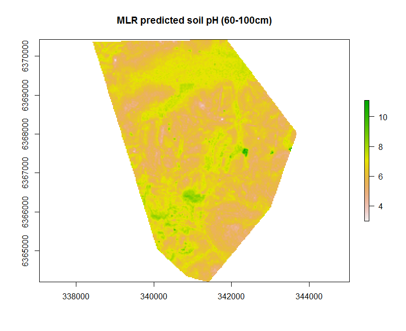
Now we can rasterise the predictions for mapping and grid export. In the example below we set the CRS to WGS84 Zone 56 before exporting the raster file out as a Geotiff file.
# create raster
map.MLR.r <- terra::rast(x = map.MLR, type = "xyz")
plot(map.MLR.r, main = "MLR predicted soil pH (60-100cm)")

# set the projection
crs(map.MLR.r) <- "+init=epsg:32756"
# write to file
terra::writeRaster(x = map.MLR.r, filename = "soilpH_60_100_MLR.tif", datatype = "FLT4S", overwrite = TRUE)
# check working directory for presence of raster
Some of the parameters used within the writeRaster function that are worth noting. The parameter datatype is specified as FLT4S which indicates that a 4 byte, signed floating point values are to be written to file. Look at the function dataType to look at other alternatives, for example for categorical data where we may be interested in logical or integer values.
Applying the model spatially using raster predict
Probably a more efficient way of applying the fitted model is to apply it directly to the rasters themselves. This avoids the step of arranging all covariates into table format. If multiple rasters are being used, it is necessary to have them arranged as a stacked SpatRaster object. This is useful as it also ensures all the rasters are of the same extent and resolution. Here we can use the terra::predict function such as below using the hv.sub.rasters as input.
# apply model to rasters directly
map.MLR.r1 <- terra::predict(object = hv.sub.rasters, model = hv.MLR.Full, filename = "soilpH_60_100_MLR.tif", datatype = "FLT4S", overwrite = TRUE)
# check working directory for presence of raster