CODE:
Get the code used in the sections about preparatory and exploratory data analysis
Intersecting soil point observations with environmental covariates
To carry out digital soil mapping in terms of evaluating the significance of environmental variables in explaining the spatial variation of the target soil variable under investigation, we need to link both sets of data together and extract the values of the covariates at the locations of the soil point data.
The first task is to bring in to our working environment some soil point data. We will be using a data set of soil samples collected from the Hunter Valley, NSW Australia. The area in question is an approximately 22km2 sub-area of the Hunter Wine Country Private Irrigation District (HWCPID), situated in the Lower Hunter Valley, NSW (32.8329S,151.354E).
The HWCPID is approximately 140 km north of Sydney, NSW, Australia. The target variable is soil pH. The data was preprocessed such that the predicted values are outputs of the mass-preserving depth function.
You will find that most examples in this section and other sections of this course that these data are used quite a bit. The data is loaded in from the ithir package with the following script:
library(ithir);library(terra);library(sf)

data(HV_subsoilpH)
str(HV_subsoilpH)

## 'data.frame':    506 obs. of  14 variables:
##  $ X                       : num  340386 340345 340559 340483 340734 ...
##  $ Y                       : num  6368690 6368491 6369168 6368740 6368964 ...
##  $ pH60_100cm              : num  4.47 5.42 6.26 8.03 8.86 ...
##  $ Terrain_Ruggedness_Index: num  1.34 1.42 1.64 1.04 1.27 ...
##  $ AACN                    : num  1.619 0.281 2.301 1.74 3.114 ...
##  $ Landsat_Band1           : int  57 47 59 52 62 53 47 52 53 63 ...
##  $ Elevation               : num  103.1 103.7 99.9 101.9 99.8 ...
##  $ Hillshading             : num  1.849 1.428 0.934 1.517 1.652 ...
##  $ Light_insolation        : num  1689 1701 1722 1688 1735 ...
##  $ Mid_Slope_Positon       : num  0.876 0.914 0.844 0.848 0.833 ...
##  $ MRVBF                   : num  3.85 3.31 3.66 3.92 3.89 ...
##  $ NDVI                    : num  -0.143 -0.386 -0.197 -0.14 -0.15 ...
##  $ TWI                     : num  17.5 18.2 18.8 18 17.8 ...
##  $ Slope                   : num  1.79 1.42 1.01 1.49 1.83 ...
As you will note, there are 506 observations of soil pH. These data are associated with a spatial coordinate and also have associated environmental covariate data that have been intersected with the point data.
The environmental covariates have been sourced from a digital elevation model and Landsat 7 satellite data. For the demonstration purposes of the exercise, we will firstly remove this already intersected data and start fresh - essentially this is an opportunity to recall earlier work on dataframe manipulation and indexing.
## Point data preparation
#round pH data to 2 decimal places
HV_subsoilpH$pH60_100cm<- round(HV_subsoilpH$pH60_100cm, 2)

#remove already intersected data
HV_subsoilpH<- HV_subsoilpH[,1:3]

#add an id column
HV_subsoilpH$id<- seq(1, nrow(HV_subsoilpH), by = 1)

#re-arrange order of columns
HV_subsoilpH<- HV_subsoilpH[,c(4,1,2,3)]

#Change names of coordinate columns
names(HV_subsoilpH)[2:3]<- c("x", "y")

# keep a record of the coordinates so they are not lost in the extraction process
HV_subsoilpH$x2<- HV_subsoilpH$x
HV_subsoilpH$y2<- HV_subsoilpH$y
Also in the ithir package are a collection of rasters that correspond to environmental covariates that cover the extent of the just loaded soil point data. These can be loaded using the script:
# locate from ithir package the rasters that are needed
hv.sub.rasters<- list.files(path = system.file("extdata/",package="ithir"),pattern = "hunterCovariates_sub",full.names = TRUE)

# read them into R as SpatRaster objects
hv.sub.rasters<- terra::rast(hv.sub.rasters)
hv.sub.rasters

## class       : SpatRaster
## dimensions  : 249, 210, 11  (nrow, ncol, nlyr)
## resolution  : 25, 25  (x, y)
## extent      : 338422.3, 343672.3, 6364203, 6370428  (xmin, xmax, ymin, ymax)
## coord. ref. : WGS 84 / UTM zone 56S (EPSG:32756)
## sources     : hunterCovariates_sub_AACN.tif
##               hunterCovariates_sub_Elevation.tif
##               hunterCovariates_sub_Hillshading.tif
##               ... and 8 more source(s)
## names       :     AACN, Elevation, Hillshading, Lands~Band1, Light~ation, Mid_S~siton, ...
## min values  :   0.0000,   72.2175,    0.000677,          26,    1236.663,    0.000009, ...
## max values  : 106.6655,  212.6325,   32.440960,         140,    1934.200,    0.956529, ...
This data set is a stack of 11 SpatRasters which correspond to mainly indices derived from a digital elevation model: elevation(elevation), terrain wetness index (TWI), altitude above channel network (AACN), terrain ruggedness index (Terrain_Ruggedness_Index), hillshading (Hillshading), incoming solar radiation (Light_insolation), mid-slope position (Mid_Slope_Positon), multi-resolution valley bottom flatness index (MRVBF), and slope gradient (Slope). Landsat 7 satellite spectral data, specifically band 1 (Landsat_Band1} and normalised difference vegetation index (NDVI) are provided too, and give some indication of the spatial variation of vegetation patterns across the study area.
Regarding the use of the list.files function above, the parameter path is essentially the directory location where the raster files are sitting. You will note the rasters come shipped with the ithir package when it is installed.
If needed, we may also want to do recursive listing into directories that are within that path directory. We want list.files() to return all the files (in our case) that have the characters hunterCovariates_sub in their file name as this excludes several other supplied files which we do not wish to use. This criteria is set via the pattern parameter. The full.names logical parameter is just a question of whether we want to return the full pathway address of the raster file, in which case, we do.
You may notice that there is a commonality between these SpatRasters in terms of their coordinate reference system (CRS), dimensions and resolution.
This harmony is an ideal situation for DSM where there may often be instances where rasters from the some area under investigation may have different resolutions, extents and even CRSs. In these situations it is common to reproject and or resample to a common projection and resolution. The functions from the terra package which may be of use in these situations are project and resample. The Reprojections, resampling and rasterisation page takes you through a number of different scenarios and workflows using these functions and others.
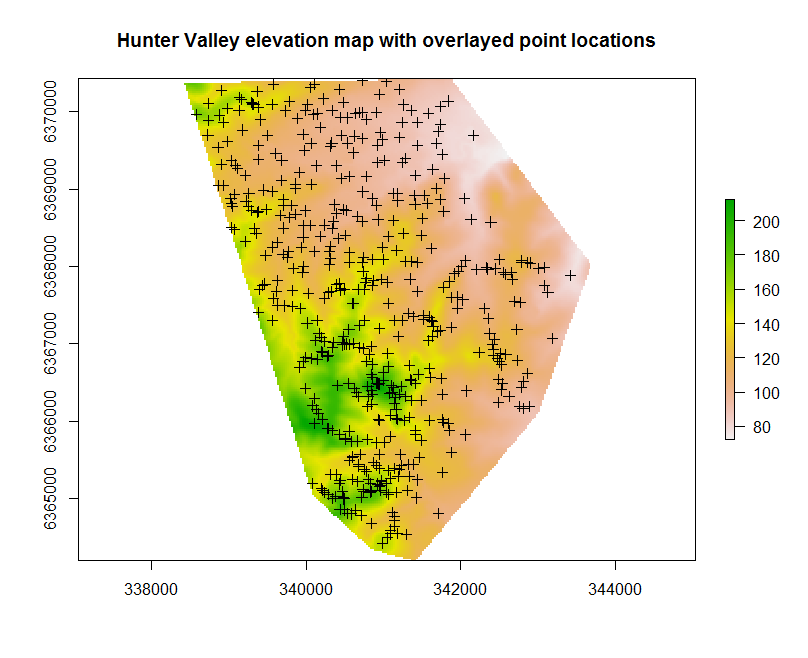
While the example is a little contrived, it is useful to always determine whether or not the available covariates have complete coverage of the soil point data. This might be done with the following script which will produce a map like in the figure below.
## plot raster
par(mfrow=c(1,1))
plot(hv.sub.rasters["Elevation"], main="Hunter Valley elevation map with overlayed point locations")

## plot points
# convert data to sf object
HV_subsoilpH <- sf::st_as_sf(x = HV_subsoilpH,coords = c("x", "y"))
plot(st_geometry(HV_subsoilpH), add=T, cex=0.5)
With the soil point data and covariates prepared, it is time to perform the intersection between the soil observations and covariate layers using the following script:
DSM_data<- terra::extract(x = hv.sub.rasters, y = HV_subsoilpH, bind = T, method = "simple")
DSM_data<- as.data.frame(DSM_data)
The extract function is quite useful. Essentially the function ingests the SpatRaster object, together with the sf object HV_subsoilpH. The bind parameter set to TRUE means that the extracted covariate data gets appended to the existing HV_subsoilpH object. For good practice, it is always helpful to retain a copy of the spatial coordinate information of your point data as it can be easily lost. This was done earlier through the creation of the x2 and y2 columns to the HV_subsoilpH data frame. A parameter from extract not used above, xy does not return the coordinates of the point data, rather the center points of the pixels where the covariate data was extracted.
The method object specifies the extraction method which in our case is simple which likened to get the covariate value nearest to the points i.e it is likened to drilling down.
A good practice is to then export the soil and covariate data intersect object to file for later use.