CODE:
Get the code used for this section here
Universal Kriging 101
- Introduction
- Data preparation
- Perform the covariate intersection
- Model fitting
- External validation
- Interpolation
Introduction
The universal kriging function in R is found in the gstat package. It is useful from the view that both the regression model and variogram modeling of the residuals are handled in one modelling system.
Using universal kriging, one can efficiently derive prediction uncertainties by way of the kriging variance. A limitation of universal kriging in the true sense of the model parameter fitting is that the model is linear.
The general preference is DSM studies is to used non-linear and recursive models that do not require strict model assumptions and assume a linear relationship between target variable and covariates.
Data preparation
So lets firstly get the data organized. Recall from before in the data preparatory exercises that we were working with the soil point data and environmental covariates for the Hunter Valley area. These data are stored in the HV_subsoilpH object together with associated rasters supplied with the ithir package.
For the succession of models examined in these various pages, we will concentrate on modelling and mapping the soil pH for the 60-100cm depth interval. To refresh, lets load the data in, then intersect the data with the available covariates.
# libraries
library(ithir)
library(MASS)
library(terra)
library(sf)
library(gstat)

# point data
data(HV_subsoilpH)

# Start afresh round pH data to 2 decimal places
HV_subsoilpH$pH60_100cm <- round(HV_subsoilpH$pH60_100cm, 2)

# remove already intersected data
HV_subsoilpH <- HV_subsoilpH[, 1:3]

# add an id column
HV_subsoilpH$id <- seq(1, nrow(HV_subsoilpH), by = 1)

# re-arrange order of columns
HV_subsoilpH <- HV_subsoilpH[, c(4, 1, 2, 3)]

# Change names of coordinate columns
names(HV_subsoilpH)[2:3] <- c("x", "y")
# save a copy of coordinates
HV_subsoilpH$x2 <- HV_subsoilpH$x
HV_subsoilpH$y2 <- HV_subsoilpH$y

# convert data to sf object
HV_subsoilpH <- sf::st_as_sf(x = HV_subsoilpH, coords = c("x", "y"))

# grids (covariate rasters from ithir package)
hv.sub.rasters <- list.files(path = system.file("extdata/", package = "ithir"), pattern = "hunterCovariates_sub", full.names = TRUE)

# read them into R as SpatRaster objects
hv.sub.rasters <- terra::rast(hv.sub.rasters)
Perform the covariate intersection
# extract covariate data
DSM_data <- terra::extract(x = hv.sub.rasters, y = HV_subsoilpH, bind = T, method = "simple")
DSM_data <- as.data.frame(DSM_data)
Often it is handy to check to see whether there are missing values both in the target variable and of the covariates. It is possible that a point location does not fit within the extent of the available covariates. In these cases the data should be excluded. A quick way to assess whether there are missing or NA values in the data is to use the complete.cases function.
which(!complete.cases(DSM_data))

## integer(0)

DSM_data <- DSM_data[complete.cases(DSM_data), ]
There do not appear to be any missing data as indicated by the integer(0) output above i.e there are zero rows with missing information.
Model fitting
First we will take a subset (using the random hold back sampling strategy) of the data to use for out-of-bag model evaluation.
# model calibration dataset
set.seed(123)
training <- sample(nrow(DSM_data), 0.7 * nrow(DSM_data))
cDat <- DSM_data[training, ]
names(cDat)[3:4] <- c("x", "y")
Now lets parametise the universal kriging model, and we will use selected covariates that were used in the multiple linear regression example.
# calculate residual variogram
vgm1 <- variogram(pH60_100cm ~ AACN + Landsat_Band1 + Elevation + Hillshading + Mid_Slope_Positon +
MRVBF + NDVI + TWI, ~x + y, data = cDat, width = 200, cutoff = 3000)

# establish some intital variogram model parameters
mod <- vgm(psill = var(cDat$pH60_100cm), "Exp", range = 3000, nugget = 0)

# fit model to residual variogram
model_1 <- fit.variogram(vgm1, mod)
model_1

##   model     psill    range
## 1   Nug 0.5386983   0.0000
## 2   Exp 0.8326639 221.5831

# plot variogram and fitted model
plot(vgm1, model = model_1)

# Universal kriging model object
gUK <- gstat(NULL, "pH", pH60_100cm ~ AACN + Landsat_Band1 + Elevation + Hillshading + Mid_Slope_Positon + MRVBF + NDVI + TWI, data = cDat, locations = ~x + y, model = model_1)
gUK

## data:
## pH : formula = pH60_100cm`~`AACN + Landsat_Band1 + Elevation + Hillshading + Mid_Slope_Positon + MRVBF + NDVI + TWI ; data dim = 354 x 13
## variograms:
##       model     psill    range
## pH[1]   Nug 0.5386983   0.0000
## pH[2]   Exp 0.8326639 221.5831
## ~x + y
External validation
Using the out-of-bag data we can evaluate the performance of universal kriging using the ithir::goof function.
## out-of-bag data
vDat <- DSM_data[-training, ]
names(vDat)[3:4] <- c("x", "y")

# make the predictions on out-of-bag data
UK.preds.V <- krige(pH60_100cm ~ AACN + Landsat_Band1 + Elevation + Hillshading +
Mid_Slope_Positon + MRVBF + NDVI + TWI, cDat, locations = ~x + y, model = model_1, newdata = vDat)

## [using universal kriging]

# evaluate UK predictions
goof(observed = DSM_data$pH60_100cm[-training], predicted = c(UK.preds.V[, 3]), plot.it = T)

##          R2 concordance   MSE     RMSE      bias
## 1 0.4381711   0.5779432 1.077 1.037786 0.0287364
The universal kriging model performs a little better than the MLR that was fitted which did not include additional spatial structure through the autocorrelation of model residuals. In the absence of additional covariate data that may help describe better the spatial properties of a given soil target variable, spatial modelling of the residuals from a deterministic model can help mop up that source of uncertainty to some extent.
Interpolation
Applying the universal kriging model spatially is facilitated through the terra::interpolate function.
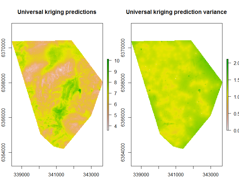
Kriging results in two main outputs: the prediction and the prediction variance.
## Apply model spatially
par(mfrow = c(1, 2))
## # prediction and prediction variance
UK.P.map <- terra::interpolate(object = hv.sub.rasters, model = gUK, xyOnly = FALSE)
plot(UK.P.map[[1]], main = "Universal kriging predictions")
plot(UK.P.map[[2]], main = "prediction variance")