CODE:
Get the code used in the sections about preparatory and exploratory data analysis
Some exploratory data analyses
Page topics
- Summary statistics
- Spatial investigations
- Inverse distance weighted interpolation
- Kriging
- Correlative data analysis
Summary statistics
We will continue using the DSM_data object that was created in Intersecting soil point observations with environmental covariates page. As the data set was saved to file you will also find it in your working directory. Type getwd() in the console to indicate the specific file location. So lets read the file in using the read.csv function. First though we need to load up a few packages to use in the following tasks. If you don’t know where the file has gotten to, use this link to download a copy.
#Load in libraries
library(ithir);library(terra);library(sf);library(gstat)
library(nortest);library(fBasics);library(ggplot2)

# load data
hv.dat <- read.csv("~/hunterValley_SoilCovariates_pH.csv")
# store copies of the cordinate data
hv.dat$x2<- hv.dat$x
hv.dat$y2<- hv.dat$y
str(hv.dat)

## 'data.frame':    506 obs. of  17 variables:
##  $ id                      : int  1 2 3 4 5 6 7 8 9 10 ...
##  $ x                       : num  340386 340345 340559 340483 340734 ...
##  $ y                       : num  6368690 6368491 6369168 6368740 6368964 ...
##  $ pH60_100cm              : num  4.47 5.42 6.26 8.03 8.86 7.28 4.95 5.61 5.39 3.44 ...
##  $ Terrain_Ruggedness_Index: num  1.34 1.42 1.64 1.04 1.27 ...
##  $ AACN                    : num  1.619 0.281 2.301 1.74 3.114 ...
##  $ Landsat_Band1           : int  57 47 59 52 62 53 47 52 53 63 ...
##  $ Elevation               : num  103.1 103.7 99.9 101.9 99.8 ...
##  $ Hillshading             : num  1.849 1.428 0.934 1.517 1.652 ...
##  $ Light_insolation        : num  1689 1701 1722 1688 1735 ...
##  $ Mid_Slope_Positon       : num  0.876 0.914 0.844 0.848 0.833 ...
##  $ MRVBF                   : num  3.85 3.31 3.66 3.92 3.89 ...
##  $ NDVI                    : num  -0.143 -0.386 -0.197 -0.14 -0.15 ...
##  $ TWI                     : num  17.5 18.2 18.8 18 17.8 ...
##  $ Slope                   : num  1.79 1.42 1.01 1.49 1.83 ...
##  $ x2                      : num  340386 340345 340559 340483 340734 ...
##  $ y2                      : num  6368690 6368491 6369168 6368740 6368964 ...
Now lets firstly look at some of the summary statistics of soil pH.
round(summary(hv.dat$pH60_100cm),1)

##    Min. 1st Qu.  Median    Mean 3rd Qu.    Max.
##     3.0     5.5     6.3     6.5     7.4     9.7
The observation that the mean and median are nearly equivalent indicates the distribution of this data does not deviate to much from normal. To assess this more formally, we can perform other analyses such as tests of skewness, kurtosis and normality. Here we need to use functions from the fBasics and nortest packages that were loaded earlier. If you do not have these already you should install them using install.packages().
# skewness
fBasics::sampleSKEW(hv.dat$pH60_100cm)

##      SKEW
## 0.1530612

# kurtosis
fBasics::sampleKURT(hv.dat$pH60_100cm)

##     KURT
## 1.202168
Here we see that the data is slightly positively skewed. A formal test for normality of the Anderson-Darling Test statistic. There are others, so its worth a look at the help files associated with the nortest package.
nortest::ad.test(hv.dat$pH60_100cm)

##
##  Anderson-Darling normality test
##
## data:  hv.dat$pH60_100cm
## A = 4.0401, p-value = 4.594e-10
For this data to be normally distributed the p value should be greater than 0.05. This is confirmed when we look at the histogram and qq-plot of this data in the figure below.
par(mfrow = c(1, 2))
hist(hv.dat$pH60_100cm)
qqnorm(hv.dat$pH60_100cm, plot.it = TRUE, pch = 4, cex = 0.7)
qqline(hv.dat$pH60_100cm, col = "red", lwd = 2)
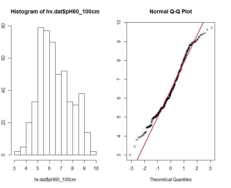
The histogram on the Figure above shows something that you would expect from a normal distribution, but in practice fails the formal statistical test. Generally for fitting most statistical models, we need to assume our data is normally distributed.
A way to make the data to be more normal is to transform it. Common transformations include the square root, logarithmic, or power transformations.
We could investigate other data transformations or even investigate the possibility of removing outliers or some such extraneous data, but generally we can be pretty satisfied with working with this data in this instance.
Spatial investigations of data
Another useful exploratory test is to visualize the data in its spatial context. Mapping the point locations with respect to the target variable by either altering the size or color of the marker gives a quick way to examine the target soil attribute spatial variability. Using the ggplot2 package, we could create the plot as shown below.
par(mfrow = c(1, 1))
ggplot2::ggplot(hv.dat, aes(x = x2, y = y2)) + geom_point(aes(size = pH60_100cm))
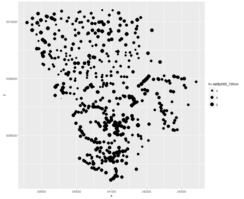
On the above figure, there is a subtle north to south trend of low to high values, but generally it is difficult to make specific observations without consideration of the terrain and landscape these data are situated in.
Ultimately we are interested in making maps. So, as a first exercise and to get a clearer sense of the spatial structure of the data it is good to use some interpolation method to estimate soil pH values onto a regular grid of the study area extent. A couple of ways of doing this is the inverse distance weighted (IDW) interpolation and kriging.
For IDW predictions, the values at unvisited locations are calculated as a weighted average of the values available at the known points, where the weights are based only by distance from the interpolation location.
Kriging is a similar distance weighted interpolation method based on values at observed locations, except it has an underlying model of the spatial variation of the data. This model is a variogram which describes the auto-correlation structure of the data as a function of distances.
Kriging is usually superior to other means of interpolation because it provides an optimal interpolation estimate for a given coordinate location, as well as a prediction variance estimate.
Kriging is very popular in soil science, and there are many variants of it. For further information and theoretical underpinnings of kriging or other associated geostatistical methods, with special emphasis for the soil sciences it is worth consulting Webster and Oliver (2001).
Inverse distance weighted interpolation
Functions for IDW interpolation and kriging are found in the gstat package.
To initiate these interpolation methods, we first need to prepare a grid of points upon which the interpolation will be made. This can be done by extracting the coordinates from either of the 25m resolution rasters we have for the Hunter Valley. As will be seen later, this step can be made redundant because we can actually interpolate directly to raster. Nevertheless, to extract the pixel point coordinates from a raster we do the following with one of the grids used earlier in the covariate intersection section. (Make sure both terra and ithir packages are loaded).
# load in from ithir the raster
hv.elevation.grid<-terra::rast(system.file("extdata/hunterCovariates_sub_Elevation.tif",package="ithir"))

# extract out coordinates for the regular grid
tempD<-data.frame(cellNos=seq(1:terra::ncell(hv.elevation.grid)))
tempD$vals<- terra::values(hv.elevation.grid)
tempD<- tempD[complete.cases(tempD),]
cellNos<- c(tempD$cellNos)
gXY<- data.frame(terra::xyFromCell(hv.elevation.grid, cellNos))
names(gXY)<- c("x2", "y2")
The script above essentially gets the pixels which have values associated with them (discards all NA occurrences), and then uses the cell numbers to extract the associated spatial coordinate locations using the xyFromCell function. The result is saved in the gXY object.
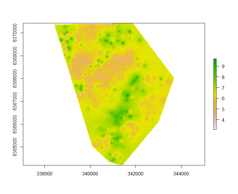
Using the idw function from gstat we fit the formula as below. We need to specify the observed data, their spatial locations, and the spatial locations of the points we want to interpolate onto.
The idp parameter allows you to specify the inverse distance weighting power. The default is 2, yet can be adjusted if you want to give more weighting to points closer to the interpolation point.
As we can not evaluate the uncertainty of prediction with IDW, we can not really optimize this parameter.
IDW.pred <- gstat::idw(hv.dat$pH60_100cm ~ 1, locations = ~x2 + y2, data = hv.dat, newdata = gXY, idp = 2)
Plotting the resulting map below can be done using the following script.
IDW.raster.p <- terra::rast(x = IDW.pred[,1:3], type = "xyz")
plot(IDW.raster.p)
Ordinary Kriging
For soil science it is more common to use kriging for the reasons that we are able to formally define the spatial relationships in our data and get an estimate of the prediction uncertainty.
As mentioned before this is done using a variogram. Variograms measure the spatial auto-correlation of phenomena such as soil properties (Pringle and McBratney 1999). The average variance between any pair of sampling points (calculated as the semi-variance) for a soil property S at any point of distance h apart can be estimated by the formula:
where γ(h) is the average semi-variance, m is the number of pairs of sampling points, s is the value of the attribute under investigation, x are the coordinates of the point, and h is the lag (separation distance of point pairs).
Therefore, in accordance with the law of geography, points closer together will show smaller semi-variance (higher correlation), whereas pairs of points farther away from each other will display larger semi-variance.
A variogram is generated by plotting the average semi-variance against the lag distance. Various models can be fitted to this empirical variogram where four of the more common ones are the linear model, the spherical model, the exponential model, and the Gaussian model.
Once an appropriate variogram has been modeled it is then used for distance weighted interpolation (kriging) at unvisited locations.
First, we calculate the empirical variogram i.e calculate the semi-variances of all point pairs in our data set.
Then we fit avariogram model (in this case we will use a spherical model).
To do this we need to make some initial estimates of this models parameters. Namely, the nugget, sill, and range.
- The nugget is the very short-range error (effectively zero distance) which is often attributed to measurement errors.
- The sill is the limit of the variogram (effectively the total variance of the data).
- The range is the distance at which the data are no longer auto-correlated.
Once we have made the first estimates of these parameters, we use the fit.variogram function for their optimization. The width parameter of the variogram function is the width of distance intervals into which data point pairs are grouped or binned for semi variance estimates as a function of distance. An automated way of estimating the variogram parameters is to use the autofitVariogram function from the automap package. For now we will stick with the gstat implementation.
vgm1 <- gstat::variogram(pH60_100cm ~ 1, ~x2 + y2, hv.dat, width = 100, cutoff = 3000)
mod <- gstat::vgm(psill = var(hv.dat$pH60_100cm), "Exp", range = 3000, nugget = 0)
model_1 <- fit.variogram(vgm1, mod)
model_1

##   model     psill    range
## 1   Nug 0.3779266   0.0000
## 2   Exp 1.5337573 353.9732
The plot in Figure below shows both the empirical variogram together with the fitted variogram model line.
plot(vgm1, model = model_1)
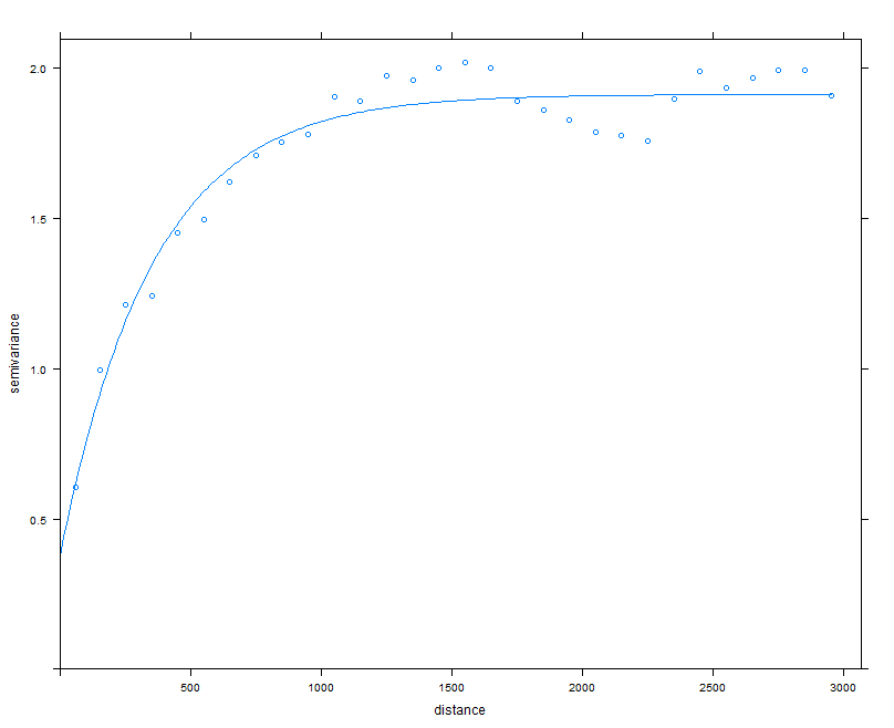
The variogram is indicating there is some spatial structure in the data up to around 500m.
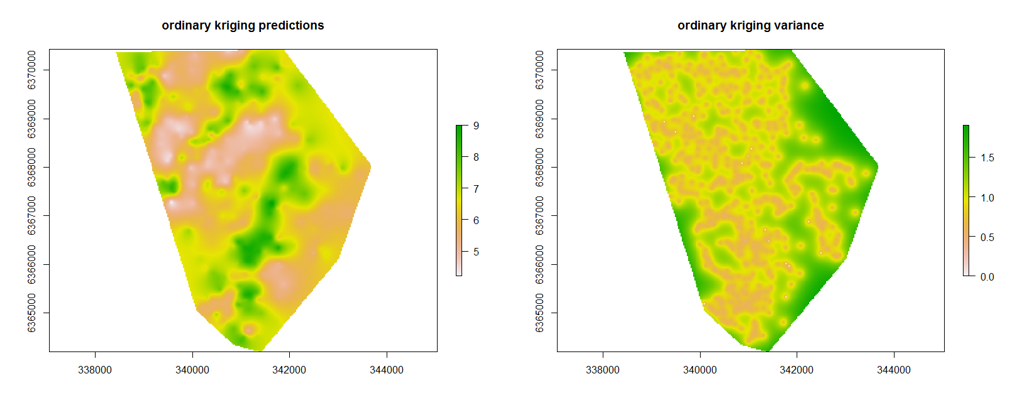
Using this fitted variogram model lets perform the kriging to make a map, but more importantly look at the variances associated with the predictions too.
Here we use the krige function, which is not unlike using idw function, except that we have the variogram model parameters as additional information.
krig.pred <- gstat::krige(hv.dat$pH60_100cm ~ 1, locations = ~x2 + y2, data = hv.dat, newdata = gXY, model = model_1)
We can make the maps as we did before, but now we can also look at the variances of the predictions too.
par(mfrow = c(2, 1))
krig.raster.p <- terra::rast(x = krig.pred[,1:3], type = "xyz")
krig.raster.var <- terra::rast(x = krig.pred[,c(1,2,4)], type = "xyz")
plot(krig.raster.p, main = "ordinary kriging predictions")
plot(krig.raster.var, main = "ordinary kriging variance")
Correlative data analysis
Understanding the geostatistical properties of the target soil variable of interest is useful in its own right. However, it is also important to determine whether there is further spatial relationships in the data that can be modeled with environmental covariate information.
Better still is to combine both spatial model approaches together (more of which will be discussed later on about this).
Ideally when we want to predict soil variables using covariate
information is that there is a reasonable correlation between them.
We can quickly assess these using the base cor function, for which we have used previously.
cor(hv.dat[, c("Terrain_Ruggedness_Index", "AACN", "Landsat_Band1",
        "Elevation", "Hillshading", "Light_insolation",
        "Mid_Slope_Positon", "MRVBF", "NDVI", "TWI", "Slope"    )],
        hv.dat[,"pH60_100cm"])

##                                  [,1]
## Terrain_Ruggedness_Index  0.146208599
## AACN                      0.194606533
## Landsat_Band1            -0.002769968
## Elevation                 0.148618926
## Hillshading               0.096981698
## Light_insolation         -0.046166532
## Mid_Slope_Positon         0.258329094
## MRVBF                     0.119674688
## NDVI                      0.162873990
## TWI                      -0.005330312
## Slope                     0.059593615
Progessing forwards later on in Continuous soil attribute modelling and mapping and Categorical soil attribute modelling and mapping, we will explore a range of models that will leverage what correlation there is between the target variable and the available covariates to create digital soil maps.
References
Pringle, M. J, and A. B McBratney. 1999. “Estimating Average and Proportional Variograms of Soil Properties and Their Potential Use in Precision Agriculture.” Precision Agriculture 1: 125–52.
Webster, R, and M. A Oliver. 2001. Geostatistics for Environmental Scientists. John Wiley; Sons Ltd, West Sussex, England.