CODE:
Get the code used for this section here
Clipping rasters
In addition to resampling and reprojecting rasters, the other common GIS task needed to harmonise different data source is to clip them to a common spatial extent. Usually the clipping is done with the extent, or bounds of another layer usually a polygon, but can be another raster too. This short piece, shows a workflow for doing this procedure in R where we have a couple of different rasters, and a polygon.
The specific raster data with which to do the exercises is found here
The specific polygon data is found here
You will need to unzip these folders to get at the data.
Initialise the libraries that are needed
library(terra);library(sf)
There are three rasters here, but for this exercise we will just use two:
files <- list.files("/~/", pattern = "tif$", full.names = T)
files

## [1] "/~/20140509.B3.tif"
## [2] "/~/elevation.tif"
## [3] "/~/GR_Th.tif"

# RASTER 1: remote sensing data
rs.raster<- terra::rast(files[1])
rs.raster

## class       : SpatRaster
## dimensions  : 3026, 4037, 1  (nrow, ncol, nlyr)
## resolution  : 0.0002245788, 0.0002245788  (x, y)
## extent      : 149.863, 150.7696, -31.64765, -30.96807  (xmin, xmax, ymin, ymax)
## coord. ref. : lon/lat WGS 84 (EPSG:4326)
## source      : 20140509.B3.tif
## name        : 20140509.B3

# RASTER 2: digital elevation model
elev.raster<- terra::rast(files[2])
elev.raster

## class       : SpatRaster
## dimensions  : 54, 81, 1  (nrow, ncol, nlyr)
## resolution  : 100, 100  (x, y)
## extent      : 1510462, 1518562, -3636821, -3631421  (xmin, xmax, ymin, ymax)
## coord. ref. : GDA94 / Geoscience Australia Lambert
## source      : elevation.tif
## name        : elevation
## min value   :  312.4171
## max value   :  590.6609
Next we load the polygon data which is called clipper_polygon.shp. The vect function comes from the terra library. The sf package may also be used to read in the polygon, but the integration of polygon tools into terra together with the usual raster tools makes for a simpler workflow.
poly.clip<- terra::vect("~/clipper_polygon.shp")
poly.clip

##  class       : SpatVector
##  geometry    : polygons
##  dimensions  : 3, 1  (geometries, attributes)
##  extent      : 150.0777, 150.152, -31.36541, -31.3309  (xmin, xmax, ymin, ymax)
##  source      : clipper_polygon.shp
##  coord. ref. : lon/lat WGS 84 (EPSG:4326)
Checking the CRS of each the the data sources, two have the same
parameters; rs.raster and poly.clip.
# CRS of data
crs(rs.raster,describe = T, proj = T)

##     name authority code area         extent                                proj
## 1 WGS 84      EPSG 4326 <NA> NA, NA, NA, NA +proj=longlat +datum=WGS84 +no_defs

crs(elev.raster, describe = T, proj = T)

##                                   name authority code area         extent
## 1 GDA94 / Geoscience Australia Lambert      <NA> <NA> <NA> NA, NA, NA, NA
##                                                                                               proj
## 1 +proj=lcc +lat_0=0 +lon_0=134 +lat_1=-18 +lat_2=-36 +x_0=0 +y_0=0 +ellps=GRS80 +units=m +no_defs

crs(poly.clip, describe = T, proj = T)

##     name authority code area         extent                                proj
## 1 WGS 84      EPSG 4326 <NA> NA, NA, NA, NA +proj=longlat +datum=WGS84 +no_defs
Below, two workflows are demonstrated.
-
Clip
rs.rasterwithpoly.clip -
Reproject the result from 1 to the same resolution and extent of
elev.raster, and also reprojectpoly.clipto this same CRS. Then clip both rasters simultaneously with the reprojected polygon.
Clip rs.raster with poly.clip
The basic workflow is to use crop, rasterize, and mask from the terra package in sequential steps to:
- Crop the raster data to extent of polygon,
- Rasterise polygon to use as a mask,
- Finalise clipping by applying the mask to the cropped raster.
# raster crop
cr <- terra::crop(rs.raster, terra::ext(poly.clip), snap="out")
# rasterise the polygon
fr <- terra::rasterize(x = poly.clip, y = cr)

# clip using mask
rs.raster.clipped <- terra::mask(x=cr, mask=fr)
We can visualise each of the steps in the below figure.

Clipping multiple rasters simultaneously
First we use terra::project to make rs.raster.clipped from above to have the same CRS, resolution and extent as elev.raster.
## reproject clipped rs.raster to same as elev.raster
rs.raster.reprojected<- terra::project(x = rs.raster.clipped, y = elev.raster, method = "bilinear")
rs.raster.reprojected

## class       : SpatRaster
## dimensions  : 54, 81, 1  (nrow, ncol, nlyr)
## resolution  : 100, 100  (x, y)
## extent      : 1510462, 1518562, -3636821, -3631421  (xmin, xmax, ymin, ymax)
## coord. ref. : GDA94 / Geoscience Australia Lambert
## source(s)   : memory
## name        : 20140509.B3
## min value   :  0.07493408
## max value   :  0.12259048
Stack the rasters to prepare both for clipping
# stack rasters
stack.rasters<- c(rs.raster.reprojected,elev.raster)
Now reproject poly.clip to the same CRS as the stack.raster object created above. Here we are using project from the terra package.
poly.clip.reprojected<- terra::project(x = poly.clip, y = crs(stack.rasters))
poly.clip.reprojected

##  class       : SpatVector
##  geometry    : polygons
##  dimensions  : 3, 1  (geometries, attributes)
##  extent      : 1510947, 1517997, -3636493, -3632217  (xmin, xmax, ymin, ymax)
##  coord. ref. : GDA94 / Geoscience Australia Lambert
##  names       :    id
##  type        : <int>
Now clipping proceeds as we did above but this time the target are the two rasters in stack.rasters.
# crop the stacked rasters to extent of polygon
cr <- terra::crop(stack.rasters, terra::ext(poly.clip.reprojected), snap="out")
# rasterise the polygon
fr <- terra::rasterize(x = poly.clip.reprojected, y = cr)
# clip using mask
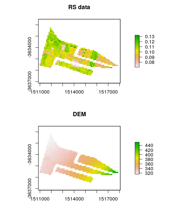
stack.rasters.clipped <- terra::mask(x=cr, mask=fr)
We can visualise both clipped rasters in the below figure.