CODE:
Get the code used for this section here
Reprojections, resampling and rasterisation
A useful thing to do in R in the GIS context are the procedures around
resampling and reprojections. Such tasks are useful in the situation of
aligning spatial data to common resolutions and extents. For digital
soil mapping this is an important and regular task to perform. Similarly
rasterisation of polygon data is another common task. This page will
cover some know-how on these topics.
- Data preparation
- Resampling
- Simultaneous reprojection and resampling
- Reprojection and resolution change
- Polygon reprojection
- Polygon rasterisation
The specific data with which to do the exercises is found here
Initialize the libraries that are needed
library(terra);library(sf)

## terra 1.7.39

##
## Attaching package: 'terra'

## The following object is masked from 'package:knitr':
##
##     spin

## Linking to GEOS 3.10.2, GDAL 3.4.3, PROJ 8.2.1; sf_use_s2() is TRUE
Data preparation
In this first part we will be working with three raster layers, each covering the same geographical area but have different projection systems, resolutions and spatial extents. After you have downloaded the data, you can use the following code to establish where they are located and retrieve the metadata of each raster.
files<- list.files("~", pattern="tif$",full.names=T)
files

## [1] "/20140509.B3.tif"
## [2] "/elevation.tif"
## [3] "/GR_Th.tif"

# RASTER 1: remote sensing data
rs.raster<- rast(files[1])
rs.raster

## class       : SpatRaster
## dimensions  : 3026, 4037, 1  (nrow, ncol, nlyr)
## resolution  : 0.0002245788, 0.0002245788  (x, y)
## extent      : 149.863, 150.7696, -31.64765, -30.96807  (xmin, xmax, ymin, ymax)
## coord. ref. : lon/lat WGS 84 (EPSG:4326)
## source      : 20140509.B3.tif
## name        : 20140509.B3

# RASTER 2: digital elevation model
elev.raster<- rast(files[2])
elev.raster

## class       : SpatRaster
## dimensions  : 54, 81, 1  (nrow, ncol, nlyr)
## resolution  : 100, 100  (x, y)
## extent      : 1510462, 1518562, -3636821, -3631421  (xmin, xmax, ymin, ymax)
## coord. ref. : GDA94 / Geoscience Australia Lambert
## source      : elevation.tif
## name        : elevation
## min value   :  312.4171
## max value   :  590.6609

# RASTER 3: Very granular gamma radiometrics data
gamma.raster<- rast(files[3])
gamma.raster

## class       : SpatRaster
## dimensions  : 606, 865, 1  (nrow, ncol, nlyr)
## resolution  : 10, 10  (x, y)
## extent      : 1510418, 1519068, -3637349, -3631289  (xmin, xmax, ymin, ymax)
## coord. ref. : +proj=lcc +lat_0=0 +lon_0=134 +lat_1=-18 +lat_2=-36 +x_0=0 +y_0=0 +ellps=GRS80 +towgs84=0,0,0,0,0,0,0 +units=m +no_defs
## source      : GR_Th.tif
## name        :    GR_Th
## min value   : 1.815541
## max value   : 8.948820
Raster resampling
The terra function to use here is resample. Here we want to get the
elev.raster to be the same resolution and extent to the
gamma.raster. Essentially going from a 100m grid cell to a 10m grid
cell. The resampling method used in bi-linear interpolation. There a
several alternative method including nearest neighbor interpolation
which is generally not appropriate for numerical data, dependent on the
context and use-case of course.
Stacking rasters is a nice feature of terra as it confirms to the user
that a collection of rasters all have the same resolution and extent.
This is really important for doing digital soil mapping. It does not
harmonise the CRS however (given the warning message below).
When rasters don’t stack, it means there is a problem, and one will have
difficulty in subsequent steps in the DSM workflow. The c function
(combine) is the tool that we need.
#resample
rs.grid<- terra::resample(x = elev.raster, y = gamma.raster, method='bilinear')
rs.grid

## class       : SpatRaster
## dimensions  : 606, 865, 1  (nrow, ncol, nlyr)
## resolution  : 10, 10  (x, y)
## extent      : 1510418, 1519068, -3637349, -3631289  (xmin, xmax, ymin, ymax)
## coord. ref. : GDA94 / Geoscience Australia Lambert
## source(s)   : memory
## name        : elevation
## min value   :  312.4536
## max value   :  590.6609

# stack
r3<- c(rs.grid, gamma.raster)

## Warning: [rast] CRS do not match

r3

## class       : SpatRaster
## dimensions  : 606, 865, 2  (nrow, ncol, nlyr)
## resolution  : 10, 10  (x, y)
## extent      : 1510418, 1519068, -3637349, -3631289  (xmin, xmax, ymin, ymax)
## coord. ref. : GDA94 / Geoscience Australia Lambert
## sources     : memory
##               GR_Th.tif
## names       : elevation,    GR_Th
## min values  :  312.4536, 1.815541
## max values  :  590.6609, 8.948820
Simultaneous reprojection and resampling
The function project is an incredibly useful function from the terra
package. As the name suggests it is used for changing data from one
projection system to another. This function also usefully does
resampling to by default where the raster (or stack of rasters) to be
processed is given the same CRS, resolution and extent as the target
raster (or stack of rasters). First, the default use case in
demonstrated, followed by a change to the target CRS but with a
resolution change.
If you recall from earlier, the rs.raster has the WGS1984 geographic
CRS: lon/lat WGS 84 (EPSG:4326), where the grid cell has a resolution
of approximately 22m, albeit expressed in decimal degrees. The target
raster is the elev.raster which has the
GDA94/ Geoscience Australia Lambert projection where the units are
expressed in meters. The resolution of this raster is 100m. Therefore in
this instance we do a reprojection and resample all in one step with the
following code. Note the use of nearest neighbor interpolation.
#reproject remote sensing grid
pl.grid <- terra::project(x =rs.raster, y = elev.raster , method="near")

# stack
r4<- c(pl.grid, elev.raster)
r4

## class       : SpatRaster
## dimensions  : 54, 81, 2  (nrow, ncol, nlyr)
## resolution  : 100, 100  (x, y)
## extent      : 1510462, 1518562, -3636821, -3631421  (xmin, xmax, ymin, ymax)
## coord. ref. : GDA94 / Geoscience Australia Lambert
## sources     : memory
##               elevation.tif
## names       : 20140509.B3, elevation
## min values  :  0.05698202,  312.4171
## max values  :  0.15245301,  590.6609
Although both rasters above stack together you will note by plotting
each raster that the remote sensing raster appears has a rectangular
extent, yet the elev.raster is clipped to some boundary. Both rasters
actually have the same extent, but for the elev.raster, part of this
data extent has no data. This is because this data is just concerned
with a particular landholding and there is not any need to have the data
surrounding it. In the exercise concerned with raster
clipping,
one can, if there is a requirement, to clip the pl.grid to the bounds
of the data in elev.raster.
Reprojection and resolution change
Rather than set the target raster to the same properties as a source
raster, one can reproject to a common CRS, but set the resolution to
what is desired. Below the rs.raster to reprojected to the the same
CRS as the elev.raster, and outputted to 50m resolution (rather than
100m as is the source raster).
#reproject and resample (50m pixels)
pl.grid50 <- terra::project(x = rs.raster, y = crs(elev.raster), method="near", res=50)
pl.grid50

## class       : SpatRaster
## dimensions  : 1701, 1888, 1  (nrow, ncol, nlyr)
## resolution  : 50, 50  (x, y)
## extent      : 1486938, 1581338, -3675127, -3590077  (xmin, xmax, ymin, ymax)
## coord. ref. : GDA94 / Geoscience Australia Lambert
## source(s)   : memory
## name        : 20140509.B3
## min value   :        - ?
## max value   :   0.5445645
Polygon reprojection
Back in the work with point patterns data you were shown how to change the CRS of sf objects. This type of transformation can also be readily extended to spatial lines and polygons too. Below, we will be working with a shapefile where the data is given as polygons, and is in fact a legacy soil map for the same geographic area as the raster data we were working with above. What we will do is load the data, do a reprojection, and a rasterisation procedure on this data. Ultimately for a digital soil mapping context we might want to use polygon data as a predictive covariate.
Now to load the data we use the st_read function from the sf package. You will note after import of the shapefile this data is encoded as a MULTIPOLYGON simple feature collection. The data frame elements of this polygon data contain the pertinent details of each polygon which in our case is descriptive information of the soil type and landscape of the area being investigated.
# read in soil map
poly.dat <- st_read("/Soils_Curlewis_GDA94.shp")

## Reading layer `Soils_Curlewis_GDA94' from data source
##   `/Soils_Curlewis_GDA94.shp'
##   using driver `ESRI Shapefile'
## Simple feature collection with 354 features and 6 fields
## Geometry type: MULTIPOLYGON
## Dimension:     XY
## Bounding box:  xmin: 150.0011 ymin: -31.49843 xmax: 150.5011 ymax: -30.99843
## Geodetic CRS:  GDA94

poly.dat

## Simple feature collection with 354 features and 6 fields
## Geometry type: MULTIPOLYGON
## Dimension:     XY
## Bounding box:  xmin: 150.0011 ymin: -31.49843 xmax: 150.5011 ymax: -30.99843
## Geodetic CRS:  GDA94
## First 10 features:
##                     NAME LANDSCAPE CODE     LENGTH   SHAPE_AREA     PROCESS
## 1        KILPHYSICS ROAD      TRkr   kr 0.06258586 1.763738e-04 TRANSFERRAL
## 2             EAST LYNNE      COel   el 0.03153234 1.838048e-05   COLLUVIAL
## 3          LONG MOUNTAIN      RElm   lm 0.03033508 1.855672e-05    RESIDUAL
## 4         QUIRINDI CREEK      ALqc   qc 0.05039743 8.478940e-05    ALLUVIAL
## 5         QUIRINDI CREEK      ALqc   qc 0.02419802 2.233679e-05    ALLUVIAL
## 6              CONADILLY      ALcd   cd 0.03408230 3.911834e-05    ALLUVIAL
## 7             BLACK JACK      REbj   bj 0.01461957 8.849160e-06    RESIDUAL
## 8  LEVER GULLY variant a     TRlga  lga 0.04916931 7.953978e-05 TRANSFERRAL
## 9             BLACK JACK      REbj   bj 0.03537858 3.183974e-05    RESIDUAL
## 10        MOUNT TAMARANG      ERmt   mt 0.25411795 8.432061e-04   EROSIONAL
##                          geometry
## 1  MULTIPOLYGON (((150.5011 -3...
## 2  MULTIPOLYGON (((150.2768 -3...
## 3  MULTIPOLYGON (((150.2766 -3...
## 4  MULTIPOLYGON (((150.4489 -3...
## 5  MULTIPOLYGON (((150.49 -31....
## 6  MULTIPOLYGON (((150.4479 -3...
## 7  MULTIPOLYGON (((150.3463 -3...
## 8  MULTIPOLYGON (((150.3993 -3...
## 9  MULTIPOLYGON (((150.2691 -3...
## 10 MULTIPOLYGON (((150.2659 -3...
Lets find out a bit more information about the poly.dat object i.e. the soil map.
# Attribute table
head(poly.dat)

##              NAME LANDSCAPE CODE     LENGTH   SHAPE_AREA     PROCESS
## 1 KILPHYSICS ROAD      TRkr   kr 0.06258586 1.763738e-04 TRANSFERRAL
## 2      EAST LYNNE      COel   el 0.03153234 1.838048e-05   COLLUVIAL
## 3   LONG MOUNTAIN      RElm   lm 0.03033508 1.855672e-05    RESIDUAL
## 4  QUIRINDI CREEK      ALqc   qc 0.05039743 8.478940e-05    ALLUVIAL
## 5  QUIRINDI CREEK      ALqc   qc 0.02419802 2.233679e-05    ALLUVIAL
## 6       CONADILLY      ALcd   cd 0.03408230 3.911834e-05    ALLUVIAL
##                         geometry
## 1 MULTIPOLYGON (((150.5011 -3...
## 2 MULTIPOLYGON (((150.2768 -3...
## 3 MULTIPOLYGON (((150.2766 -3...
## 4 MULTIPOLYGON (((150.4489 -3...
## 5 MULTIPOLYGON (((150.49 -31....
## 6 MULTIPOLYGON (((150.4479 -3...

# soil type code and frequency
summary(poly.dat)

##      NAME            LANDSCAPE             CODE               LENGTH
##  Length:354         Length:354         Length:354         Min.   :0.004702
##  Class :character   Class :character   Class :character   1st Qu.:0.020827
##  Mode  :character   Mode  :character   Mode  :character   Median :0.042751
##                                                           Mean   :0.144449
##                                                           3rd Qu.:0.133895
##                                                           Max.   :2.620946
##    SHAPE_AREA          PROCESS                   geometry
##  Min.   :3.800e-07   Length:354         MULTIPOLYGON :354
##  1st Qu.:1.665e-05   Class :character   epsg:4283    :  0
##  Median :6.608e-05   Mode  :character   +proj=long...:  0
##  Mean   :7.062e-04
##  3rd Qu.:3.658e-04
##  Max.   :3.170e-02

summary(as.factor(poly.dat$CODE)) # numeric factor

##  bh  bj  bo  ca  cd  cr  cu  dh  el  fr  gi  gl  go  gy  ha  kr  lg lga  lm  lo
##  18  26   9  10  16  12   1   2  12  12   6   4  16   3   2   1   2   2  13  14
##  lr  ma  md  mm  mn  mo  mt  mw  nj  ph  pn  po  qc  sg  ta  tf  tu  wa wfa  xx
##   3   1   1  17   2   4   6   2   9  12  10   8  13  29   5   7  11  10   1  21
##  ya
##   1

#Basic plot
plot(poly.dat)

# coordinate reference system
st_crs(poly.dat)

## Coordinate Reference System:
##   User input: GDA94
##   wkt:
## GEOGCRS["GDA94",
##     DATUM["Geocentric Datum of Australia 1994",
Currently the data is in GDA94 CRS: Geocentric Datum of Australia 1994, and we want to have it in the projected GDA94 / Geoscience Australia Lambert system as for the
rasters that were processed above.
## Reproject to new projection (newProj)
newProj<- st_crs(pl.grid)
poly.dat.T <- st_transform(poly.dat, crs= newProj)
poly.dat.T

## Simple feature collection with 354 features and 6 fields
## Geometry type: MULTIPOLYGON
## Dimension:     XY
## Bounding box:  xmin: 1501899 ymin: -3655548 xmax: 1555750 ymax: -3595023
## Projected CRS: GDA94 / Geoscience Australia Lambert
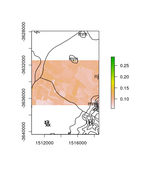
To confirm this worked we can plot the remote sensing grid (pl.grid50)
and overlay the polygon data.
plot(pl.grid)
plot(poly.dat.T["LANDSCAPE"], add = T, col = sf.colors(categorical = TRUE, alpha = 0.2))
Rasterisation
The function we need here is rasterize from the terra package. First
the sf object need to be coherced to a terra data type which is a
SpatVector. Here we will rasterise the CODE variable of the polygon
data, and fit it to the same resolution and extent as the pl.grid50
remote sensing data.
# convert sf to vect
poly.dat.V<- terra::vect(poly.dat.T)

# rasterise
poly.raster <- terra::rasterize(x = poly.dat.V, y = pl.grid50, field="CODE")
names(poly.raster)<- "soil_map_CODE"

#stack
r5<- c(pl.grid50,poly.raster)
r5

## class       : SpatRaster
## dimensions  : 1701, 1888, 2  (nrow, ncol, nlyr)
## resolution  : 50, 50  (x, y)
## extent      : 1486938, 1581338, -3675127, -3590077  (xmin, xmax, ymin, ymax)
## coord. ref. : GDA94 / Geoscience Australia Lambert
## source(s)   : memory
## names       : 20140509.B3, soil_map_CODE
## min values  :        - ? ,            bh
## max values  :   0.5445645,            ya