CODE:
Get the code used for this section here
Working with raster data
Most of the functions needed for handling raster data are contained in the terra package. There are functions for reading and writing raster files from and to different raster formats. In DSM we work quite a deal with data in table format and then rasterise this data so that we can make a map. To do this in R, lets bring in a data.frame. This could be either from a text-file, but as for the previous occasions, the data is imported from the ithir package. This data is a digital elevation model with 100m grid resolution, from the Hunter Valley, NSW, Australia. The same area where the data point pattern used in the point patterns page originated from.
library(ithir)
data(HV_dem)
str(HV_dem)

## 'data.frame':    21518 obs. of  3 variables:
##  $ X        : num  340210 340310 340110 340210 340310 ...
##  $ Y        : num  6362640 6362640 6362740 6362740 6362740 ...
##  $ elevation: num  177 175 178 172 173 ...
As the data is already a raster (such that the row observation
indicate locations on a regular spaced grid), but in a table format, we can just use the rast function from terra with an additional specification for the type argument stating it is of type xyz, simply saying, if the value is xyz, the data must have at least two columns, the first with x (or longitude) and the second with y (or latitude) coordinates that represent the centers of raster cells. The additional columns are the values associated with the raster cells.
Additionally we can define the CRS just like we did with the HV100 point data we worked with before.
r.DEM <- terra::rast(x = HV_dem, type = "xyz")
crs(r.DEM) <- "+init=epsg:32756"
r.DEM

## class       : SpatRaster
## dimensions  : 215, 169, 1  (nrow, ncol, nlyr)
## resolution  : 100, 100  (x, y)
## extent      : 334459.8, 351359.8, 6362590, 6384090  (xmin, xmax, ymin, ymax)
## coord. ref. : WGS 84 / UTM zone 56S
## source(s)   : memory
## name        : elevation
## min value   :  29.61407
## max value   : 315.68365
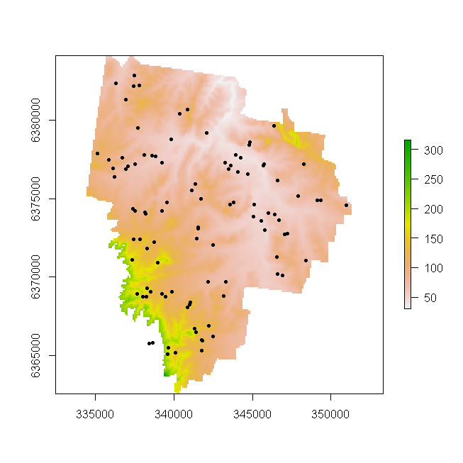
So lets do a quick plot of this raster and overlay the HV100 point locations. (Note you will have needed to process the HV100 data accordingly as per the point patterns page to show this figure).
plot(r.DEM)
points(HV100, pch = 20)
So we may want to export this raster to a suitable format for further work in a standard GIS environment. See the help file for writeRaster to get information regarding the supported grid types that data can be exported. For demonstration, we will export our data to GeoTIFF format, as this is widely used and well supported format.
terra::writeRaster(x = r.DEM, filename = "HV_dem100.tif", overwrite = TRUE)
What about reprojecting this raster to another CRS. For example,
currently the data is in WGS 84 / UTM zone 56S CRS, yet we might want it in WGS 84 geographic projection. Raster reprojection is performed using the project function from terra. Look at the help file for this function. The x argument takes the raster we wish to reproject. The y argument can take another raster that has the CRS we want to reproject to, or simply the CRS description. Another important argument
is method which controls the interpolation method. For continuous data, bilinear would be suitable, but for categorical, ngb, (which is nearest neighbor interpolation) is probably better suited. Some more information and applications of the projectRaster function can be found in the Raster resampling and reprojections page.
p.r.DEM <- terra::project(x = r.DEM, y = "+init=epsg:4326", method = "bilinear")
p.r.DEM

## class       : SpatRaster
## dimensions  : 203, 191, 1  (nrow, ncol, nlyr)
## resolution  : 0.0009657863, 0.0009657863  (x, y)
## extent      : 151.2308, 151.4152, -32.86451, -32.66845  (xmin, xmax, ymin, ymax)
## coord. ref. : lon/lat WGS 84
## source(s)   : memory
## name        : elevation
## min value   :  29.91465
## max value   : 312.51022
The other useful procedure we can perform is to import rasters directly into R so we can perform further analyses.
read.grid <- rast("HV_dem100.tif")
read.grid

## class       : SpatRaster
## dimensions  : 215, 169, 1  (nrow, ncol, nlyr)
## resolution  : 100, 100  (x, y)
## extent      : 334459.8, 351359.8, 6362590, 6384090  (xmin, xmax, ymin, ymax)
## coord. ref. : WGS 84 / UTM zone 56S (EPSG:32756)
## source      : HV_dem100.tif
## name        : elevation
## min value   :  29.61407
## max value   : 315.68365
The imported raster read.grid is a SpatRaster object.
You will notice from the R generated output indicating the data
source. Currently this source of the GeoTIFF, but alternatively it might also be loaded into the R memory, which is great for small files. A really powerful feature of the terra package is the ability to point to the location of a raster/s without the need to load it into memory.
It is only very rarely that one needs to use all the data contained in a raster at one time. As will be seen later on, this useful feature makes for a very efficient way to perform digital soil mapping across very large spatial extents.