CODE:
Get the code used for this section here
Uncertainty estimation based on local errors and data partitioning
- Pre-work reading
- Defining the model parameters
- Within ruleset prediction limits
- Mapping predictions and model uncertainties
- Evaluating the quantification of uncertainties
Pre-work reading
The approach for uncertainty quantification described here and in further section are empirical methods whereby the prediction intervals are defined from the distribution of underlying model errors i.e. the deviation between observation and model predictions.
In other types of uncertainty quantification, the prediction limits are not spatially uniform as they are for bootstrap uncertainty quantification. Rather they are a function of the landscape. For example, in some areas of the landscape, or in some particular landscape situations, the prediction is going to be more accurate than in other situations.
For the immediate approach, an explicit landscape partition is used to define likely areas where the quantification of uncertainty may differ. This approach uses the Cubist data mining algorithm for prediction and partitioning of the landscape. Within each partitioned area, we can then define the distribution of model errors.
This approach for uncertainty quantification was used by Malone et al. (2014) where soil pH was predicted using a Cubist model and residual kriging spatial model.
This approach and the fuzzy clustering approach are useful from the viewpoint that complex models in terms of parameterisation) are able to be used within a digital soil mapping framework where there is a necessity to define a stated level of prediction confidence.
With universal kriging, this is the restriction of the linear model (which in many situations could be the best model). For empirical approaches to uncertainty quantification, this restriction does not exist. Further to this, the localized allocation of prediction limits i.e. in given landscape situations provides a means to identify areas where mapping is accurate and where it is not so much. Often this is a function of the sampling density. This explicit allocation of prediction intervals may assist with the future design of soil sampling programs.
In the approach to be described, the partitioning is a “hard” partition as opposed to a ‘soft’ or ‘fuzzy’ partition approach.
Defining the model parameters
In this example we will use the Cubist model regression model, and then define the subsequent prediction intervals.
First we load libraries, data and then prepare it for analysis.
# Libraries
library(ithir)
library(MASS)
library(sf)
library(terra)
library(Cubist)

# point data
data(HV_subsoilpH)

# Start afresh round pH data to 2 decimal places
HV_subsoilpH$pH60_100cm <- round(HV_subsoilpH$pH60_100cm, 2)

# remove already intersected data
HV_subsoilpH <- HV_subsoilpH[, 1:3]

# add an id column
HV_subsoilpH$id <- seq(1, nrow(HV_subsoilpH), by = 1)

# re-arrange order of columns
HV_subsoilpH <- HV_subsoilpH[, c(4, 1, 2, 3)]

# Change names of coordinate columns
names(HV_subsoilpH)[2:3] <- c("x", "y")
# save a copy of coordinates
HV_subsoilpH$x2 <- HV_subsoilpH$x
HV_subsoilpH$y2 <- HV_subsoilpH$y

# convert data to sf object
HV_subsoilpH <- sf::st_as_sf(x = HV_subsoilpH, coords = c("x", "y"))

# grids (covariate rasters from ithir package)
hv.sub.rasters <- list.files(path = system.file("extdata/", package = "ithir"), pattern = "hunterCovariates_sub",
full.names = TRUE)

# read them into R as SpatRaster objects
hv.sub.rasters <- terra::rast(hv.sub.rasters)

# extract covariate data
DSM_data <- terra::extract(x = hv.sub.rasters, y = HV_subsoilpH, bind = T, method = "simple")
DSM_data <- as.data.frame(DSM_data)

# check for NA values
which(!complete.cases(DSM_data))

## integer(0)

DSM_data <- DSM_data[complete.cases(DSM_data), ]

# subset data for modeling
set.seed(1000)
training <- sample(nrow(DSM_data), 0.7 * nrow(DSM_data))
DSM_data_cal <- DSM_data[training, ]  # calibration
DSM_data_val <- DSM_data[-training, ]  # validation
Note that the nature of the data sometimes make demonstration of an example a little difficult. Subsequently, some prior analysis was performed of the model fitting in order to ensure that at least one data partition was formed. Therefore using the below data configuration as defined through the set.seed(1000) randomisation setting and specific covariate data selections should yield two cubist model partitions or rulesets.
# Cubist model
hv.cub.Exp <- cubist(x = DSM_data_cal[, c(5, 11, 13, 15)], y = DSM_data_cal$pH60_100cm,
cubistControl(unbiased = TRUE, rules = 10, extrapolation = 5, sample = 0, label = "outcome"), committees = 1)

summary(hv.cub.Exp)

##
## Call:
## cubist.default(x = DSM_data_cal[, c(5, 11, 13, 15)], y
##  = DSM_data_cal$pH60_100cm, committees = 1, control = cubistControl(unbiased
##  = TRUE, rules = 10, extrapolation = 5, sample = 0, label = "outcome"))
##
##
## Cubist [Release 2.07 GPL Edition]  Wed Sep 20 22:20:07 2023
## ---------------------------------
##
##     Target attribute `outcome'
##
## Read 354 cases (5 attributes) from undefined.data
##
## Model:
##
##   Rule 1: [336 cases, mean 6.443, range 3.44 to 9.74, est err 1.025]
##
##     if
##  MRVBF > 0.004846
##     then
##  outcome = 3.978 + 0.028 AACN + 0.38 MRVBF + 0.082 TWI + 0.04 Slope
##
##   Rule 2: [18 cases, mean 8.018, range 6.26 to 9.45, est err 0.434]
##
##     if
##  MRVBF <= 0.004846
##     then
##  outcome = 8.686 + 471.23 MRVBF - 0.0236 AACN
##
##
## Evaluation on training data (354 cases):
##
##     Average  |error|              1.222
##     Relative |error|               1.08
##     Correlation coefficient        0.22
##
##
##  Attribute usage:
##    Conds  Model
##
##    100%   100%    MRVBF
##           100%    AACN
##            95%    Slope
##            95%    TWI
##
##
## Time: 0.0 secs
Assessing the goodness of fit of this model, we use the goof function.
## goodness of fit (calibration)
goof(observed = DSM_data_cal$pH60_100cm, predicted = predict(hv.cub.Exp, newdata = DSM_data_cal))

##          R2 concordance      MSE     RMSE         bias
## 1 0.2088674   0.3432409 1.458209 1.207563 0.0001963093
Two things we want to save from this process are the model residuals and the expression for each data case as to which partition or ruleset it belongs to. To do this second step we need to take note of the partitioning variables and their threshold values and use indexing to attribute each case to its ruleset.
# append rule specification to data
DSM_data_cal$rule_spec <- NA
DSM_data_cal$rule_spec[which(DSM_data_cal$MRVBF > 0.004846)] <- 1
DSM_data_cal$rule_spec[which(DSM_data_cal$MRVBF <= 0.004846)] <- 2

## Model residuals
DSM_data_cal$residual <- DSM_data_cal$pH60_100cm - predict(hv.cub.Exp, newdata = DSM_data_cal)
Within ruleset prediction limits
With a model defined, it is now necessary to estimate the within partition prediction limits. While we may only want to map the lower 5th and upper 95th prediction limits, we also want to get at the sensitivity of the uncertainty quantifications which calls for the evaluation of quantiles for a range of confidence levels (in this case sequentially from 5% to 99%) for calculation of the PICP. This is done using the quantile function and is performed for each ruleset.
# distribution of residuals in each rule set
hist(DSM_data_cal$residual[DSM_data_cal$rule_spec == 1], main = "Residuals ruleset 1")

hist(DSM_data_cal$residual[DSM_data_cal$rule_spec == 2], main = "Residuals ruleset 2")

# Quantiles of residual distribution within each ruleset Rule 1
r1.q <- quantile(DSM_data_cal$residual[DSM_data_cal$rule_spec == 1], probs = c(0.005, 0.995, 0.0125, 0.9875, 0.025, 0.975, 0.05, 0.95, 0.1, 0.9, 0.2, 0.8, 0.3, 0.7, 0.4, 0.6, 0.45, 0.55, 0.475, 0.525), na.rm = FALSE, names = T, type = 7)
r1.q

##        0.5%       99.5%       1.25%      98.75%        2.5%       97.5%
## -2.35907828  3.18669415 -2.11623531  3.10336920 -1.90018377  2.91098968
##          5%         95%         10%         90%         20%         80%
## -1.69229583  2.44896853 -1.39467810  1.77711057 -1.05917666  1.03383651
##         30%         70%         40%         60%         45%         55%
## -0.79152037  0.59774065 -0.56821804  0.15932105 -0.35169148 -0.01512939
##       47.5%       52.5%
## -0.29393916 -0.12533224

# Rule 2
r2.q <- quantile(DSM_data_cal$residual[DSM_data_cal$rule_spec == 2], probs = c(0.005, 0.995, 0.0125, 0.9875, 0.025, 0.975, 0.05, 0.95, 0.1, 0.9, 0.2, 0.8, 0.3, 0.7, 0.4, 0.6, 0.45, 0.55, 0.475, 0.525), na.rm = FALSE, names = T, type = 7)
r2.q

##        0.5%       99.5%       1.25%      98.75%        2.5%       97.5%
## -0.91812929  0.78924818 -0.85184640  0.73841167 -0.74137491  0.65368415
##          5%         95%         10%         90%         20%         80%
## -0.52043193  0.48422911 -0.37243120  0.36673757 -0.29524641  0.17231533
##         30%         70%         40%         60%         45%         55%
## -0.16111519  0.13421975 -0.05547775  0.10625404  0.05552533  0.09982510
##       47.5%       52.5%
##  0.09317083  0.09703764
Despite many more cases belong to one ruleset compared to the other, the prediction limits for each partition of the data are quite different from each other. This goes some way to understanding that prediction uncertainty ranges are certainly not spatially uniform. In some areas of the landscape we might expect to predict some soil attribute rather accurately, but in other landscape positions the relationships are more complex.
Mapping predictions and model uncertainties
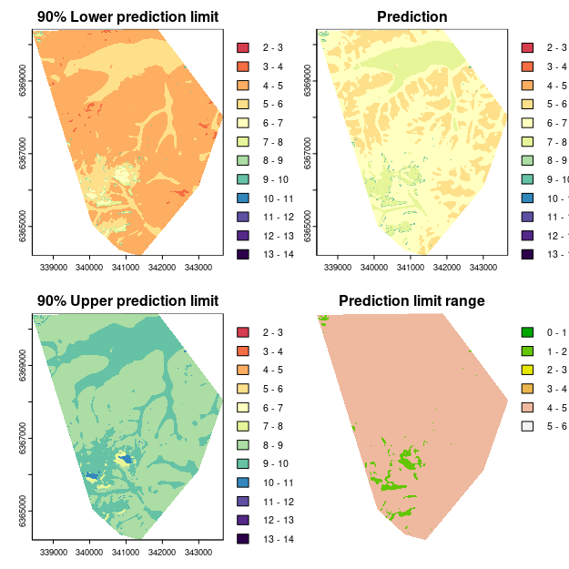
The creation of the model prediction map brings no new surprises in approach. For the mapping of prediction limits however, we basically need to partition the map area based on the given variables and their thresholds, and then within each area, apply the specific model error ranges for the 90% confidence level. The terra::ifel function is particularly helpful in advancing this process.
## MAPPING cubist model prediction
map.cubist <- terra::predict(object = hv.sub.rasters, model = hv.cub.Exp)

# note there is a need to mask are the area outside soil mapping boundary
msk <- terra::ifel(is.na(hv.sub.rasters[[1]]), NA, 1)
map.cubist <- terra::mask(map.cubist, msk, inverse = F)

# map the rule set distribution
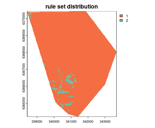
mapped.ruleset <- ifel(hv.sub.rasters[["MRVBF"]] > 0.004846, 1, 2)

# upper and lower prediction intervals upper
map.cubist.upl <- terra::ifel(mapped.ruleset == 1, map.cubist + r1.q[8], map.cubist + r2.q[8])

# lower
map.cubist.lpl <- terra::ifel(mapped.ruleset == 1, map.cubist + r1.q[7], map.cubist + r2.q[7])

# Prediction interval range
map.cubist.pir <- map.cubist.upl - map.cubist.lpl
Plotting each of the maps.
## color ramp
phCramp <- c("#d53e4f", "#f46d43", "#fdae61", "#fee08b", "#ffffbf", "#e6f598", "#abdda4", "#66c2a5", "#3288bd", "#5e4fa2", "#542788", "#2d004b")
brk <- c(2:14)
par(mfrow = c(2, 2))

plot(map.cubist.lpl, main = "90% Lower prediction limit", breaks = brk, col = phCramp)
plot(map.cubist, main = "Prediction", breaks = brk, col = phCramp)
plot(map.cubist.upl, main = "90% Upper prediction limit", breaks = brk, col = phCramp)
plot(map.cubist.pir, main = "Prediction limit range", col = terrain.colors(length(seq(0, 6.5, by = 1)) - 1), axes = FALSE, breaks = seq(0, 6.5, by = 1))

For interests sake the map of the spatial distribution of each ruleset is shown below. Only a relatively small area is attributed to ruleset 2.

Evaluating the quantification of uncertainties
For out-of-bag model evaluation we assess both the quality of the predictions and the quantification of uncertainty. Below we assess the validation of the cubist model.
## Model evaluation with out-of-bag cases Cubist model prediction
DSM_data_val$model_pred <- predict(hv.cub.Exp, newdata = DSM_data_val)

# Evaluation
goof(observed = DSM_data_val$pH60_100cm, predicted = DSM_data_val$model_pred)

##          R2 concordance      MSE    RMSE       bias
## 1 0.1387573    0.274822 1.494898 1.22266 0.09989099
The first step in estimating the uncertainty about the validation points is to evaluate which ruleset each case belongs to.
# append rule specification to data
DSM_data_val$rule_spec <- NA
DSM_data_val$rule_spec[which(DSM_data_val$MRVBF > 0.004846)] <- 1
DSM_data_val$rule_spec[which(DSM_data_val$MRVBF <= 0.004846)] <- 2
summary(as.factor(DSM_data_val$rule_spec))

##   1   2
## 145   7
Then we can define the prediction interval that corresponds to each observation for each level of confidence.
# upper and lower prediction limits upper
ulMat <- matrix(NA, nrow = nrow(DSM_data_val), ncol = length(r1.q))
for (i in seq(2, 20, 2)) {
ulMat[which(DSM_data_val$rule_spec == 1), i] <- r1.q[i]
ulMat[which(DSM_data_val$rule_spec == 2), i] <- r2.q[i]}

# lower
for (i in seq(1, 20, 2)) {
ulMat[which(DSM_data_val$rule_spec == 1), i] <- r1.q[i]
ulMat[which(DSM_data_val$rule_spec == 2), i] <- r2.q[i]}

# upper and lower prediction limits
ULpreds <- ulMat + DSM_data_val$model_pred
ULpreds <- as.data.frame(ULpreds)
names(ULpreds) <- names(r1.q)
DSM_data_val <- cbind(DSM_data_val, ULpreds)
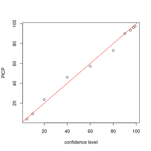
The PICP estimates appear to correspond quite well with the respective confidence levels. This can be observed from the plot on Figure below too.
# PICP
bMat <- matrix(NA, nrow = nrow(ULpreds), ncol = (ncol(ULpreds)/2))
cnt <- 1
for (i in seq(1, 20, 2)) {
bMat[, cnt] <- as.numeric(DSM_data_val$pH60_100cm <= ULpreds[, i + 1] & DSM_data_val$pH60_100cm >= ULpreds[, i])
cnt <- cnt + 1}

# plotting
par(mfrow = c(1, 1))
cs <- c(99, 97.5, 95, 90, 80, 60, 40, 20, 10, 5)
plot(cs, ((colSums(bMat)/nrow(bMat)) * 100), ylab = "PICP", xlab = "confidence level")
# draw 1:1 line
abline(a = 0, b = 1, col = "red")

Looking at the quantiles of the prediction interval ranges we can see the effect that data partitioning has which is distinct grouping of the uncertainty.
quantile(ULpreds[, 8] - ULpreds[, 7])

##       0%      25%      50%      75%     100%
## 1.004661 4.141264 4.141264 4.141264 4.141264
The demonstration of this method may not be too helpful with the data at hand, and this example should only be used for illustration of concept rather than as a promotion or demotion of the method. Due to the relatively small number of cases in ruleset 2 compared with ruleset 1, we might expect to observe clear differences in the confidence in the uncertainty quantification between the different rulesets.
# PICP by rule set for 90% confidence rule 1
sum(DSM_data_val$pH60_100cm[DSM_data_val$rule_spec == 1] <= DSM_data_val$`95%`[DSM_data_val$rule_spec == 1] & DSM_data_val$pH60_100cm[DSM_data_val$rule_spec == 1] >= DSM_data_val$`5%`[DSM_data_val$rule_spec == 1])/nrow(DSM_data_val[DSM_data_val$rule_spec == 1, ])

## [1] 0.9241379

# rule 2
sum(DSM_data_val$pH60_100cm[DSM_data_val$rule_spec == 2] <= DSM_data_val$`95%`[DSM_data_val$rule_spec == 2] & DSM_data_val$pH60_100cm[DSM_data_val$rule_spec == 2] >= DSM_data_val$`5%`[DSM_data_val$rule_spec == 2])/nrow(DSM_data_val[DSM_data_val$rule_spec == 2, ])

## [1] 0.4285714
Despite the small number of cases in ruleset two, we can still be encouraged that just under half the cases fit within their relatively narrow prediction envelopes for the 90% confidence level.
References
Malone, B P, B Minasny, N P Odgers, and A B McBratney. 2014. “Using Model Averaging to Combine Soil Property Rasters from Legacy Soil Maps and from Point Data.” Geoderma 232-234: 34–44.