CODE:
Get the code used for this section here
C5 decision trees
Introduction
The C5 decision tree model is available in the C50 package. The function C5.0 fits classification tree models or rule-based models using Quinlans’s C5.0 algorithm (Quinlan 1993).
Essentially we will go through the same process as we did for the multinomial logistic regression.
The C5.0 function and its internal parameters are similar in nature to that of the Cubist function for predicting continuous variables. The trials parameter lets you implement a boosted classification tree process, with the results aggregated at the end. There are also many other useful model tuning parameters in the C5.0Control parameter set too that are worth a look. Just see the help files for more information.
Data Preparation
The data to be used for the following modelling exercises are Terron classes as sampled from the map presented in Malone et al. (2014). The sample data contains 1000 cases of which there are 12 different Terron classes. Before getting into the modeling, we first load in the data and then perform the covariate layer intersection using the suite of environmental variables sourced from the ithir package.
The small selection of covariates cover an area of approximately 220km2 at a spatial resolution of 25m. All these variables are derived primarily from an available digital elevation model.
## load libraries
library(ithir)
library(sf)
library(terra)
library(C50)

# point data of terron classifications
data(hvTerronDat)

# environmental covariates grids (covariate rasters from ithir package)
hv.rasters <- list.files(path = system.file("extdata/", package = "ithir"), pattern = "hunterCovariates_A", full.names = T)
hv.rasters

# read them into R as SpatRaster objects
hv.rasters <- terra::rast(hv.rasters)
Transform the hvTerronDat data to a sf object or simple feature collection which will permit spatial analysis to take place.
## coerce point data to spatial object
hvTerronDat <- sf::st_as_sf(x = hvTerronDat, coords = c("x", "y"))
As these data are of the same spatial projection as the raster data, there is no need to perform a coordinate transformation. So we can perform the intersection immediately.
## Covariate data extraction
DSM_data <- terra::extract(x = hv.rasters, y = hvTerronDat, bind = T, method = "simple")
DSM_data <- as.data.frame(DSM_data)
str(DSM_data)

## 'data.frame':    1000 obs. of  9 variables:
It is always good practice to check to see if any of the observational data returned any NA values for any one of the covariates. If there is NA values, it indicates that the observational data is outside the extent of the covariate layers. It is best to remove these observations from the data set.
## remove missing data
which(!complete.cases(DSM_data))

## integer(0)

DSM_data <- DSM_data[complete.cases(DSM_data), ]
We will also subset the data for an external validation i.e. random hold back validation. Here 70% of the data for model calibration, leaving the other 30% for validation.
## Random holdback
set.seed(655)
training <- sample(nrow(DSM_data), 0.7 * nrow(DSM_data))
Model fitting
With the calibration data prepared, we will fit the C5 model as in the script below.
hv.C5 <- C5.0(x = DSM_data[training, 2:9], y = DSM_data$terron[training], trials = 1, rules = FALSE, control = C5.0Control(CF = 0.95, minCases = 20, earlyStopping = FALSE))
By calling the summary function, some useful model fit diagnostics are given. These include the tree structure, together with the covariates used and mis-classification error of the model, as well as a rudimentary confusion matrix. A useful feature of the C5 model is that it can omit in an automated fashion, unnecessary covariates.
The predict function can either return the predicted class or the confidence of the predictions (which is controlled using the type= prob parameter. The probabilities are quantified such that if an observation is classified by a single leaf of a decision tree, the confidence value is the proportion of training cases at that leaf that belong to the predicted class. If more than one leaf is involved (i.e. one or more of the attributes on the path has missing values), the value is a weighted sum of the individual leaves’ confidences.
For rule-classifiers, each applicable rule votes for a class with the voting weight being the rule’s confidence value. If the sum of the votes for class C is W(C), then the predicted class P is chosen so that W(P) is maximal, and the confidence is the greater of (1), the voting weight of the most specific applicable rule for predicted class P; or (2) the average vote for class P (so, W(P) divided by the number of applicable rules for class P).Boosted classifiers are similar, but individual classifiers vote for a class with weight equal to their confidence value. Overall, the confidence associated with each class for every observation are made to sum to 1.
# return the class predictions
predict(hv.C5, newdata = DSM_data[training, ])[1:10]

##  [1] 3 8 8 5 7 5 5 6 8 5
## Levels: 1 2 3 4 5 6 7 8 9 10 11 12

# return the class probabilities (Terron classes 1 to 3, first 10 cases)
predict(hv.C5, newdata = DSM_data[training, ], type = "prob")[1:10, 1:3]

##                1            2            3
## 366 0.0002918587 1.382488e-04 0.4742242759
## 79  0.0001675485 7.936508e-05 0.0006349206
## 946 0.0001675485 7.936508e-05 0.0006349206
## 148 0.0007983193 3.781512e-04 0.0030252100
## 710 0.0006031746 2.857143e-04 0.3133968224
## 729 0.0011309523 5.357143e-04 0.0042857142
## 848 0.0003270224 1.549053e-04 0.0012392427
## 20  0.0010052910 4.761905e-04 0.0038095239
## 923 0.0001675485 7.936508e-05 0.0006349206
## 397 0.0003270224 1.549053e-04 0.0012392427
Model goodness of fit
So lets look at the calibration and out-of-bag model goodness of fit evaluations. First, the calibration statistics:
## Goodness of fit calibration data
C.pred.hv.C5 <- predict(hv.C5, newdata = DSM_data[training, ])
goofcat(observed = DSM_data$terron[training], predicted = C.pred.hv.C5)

## $confusion_matrix
##     1 2  3  4  5  6  7  8  9 10 11 12
## 1  16 3  0  5  0  0  0  0  2  1  0  0
## 2   0 0  0  0  0  0  0  0  0  0  0  0
## 3   0 6 54  1  0  0 16  2  0  2 14 17
## 4   0 0  1 12  0  0  3  1  3  1  0  0
## 5   0 0  0  2 82  9  9  1 12 18  3  2
## 6   0 0  0  0  4 46  0  0  0  1  0  0
## 7   0 0 17 10  0  0 70 12  6 10  3 14
## 8   0 0  0  4  4  9 24 89  8 12 11  0
## 9   3 0  0  9  0  0  0  0 15  0  0  0
## 10  0 0  0  0  2  3  0  4  0  9  2  1
## 11  0 0  0  0  0  0  0  0  0  0  0  0
## 12  0 0  0  0  0  0  0  0  0  0  0  0
##
## $overall_accuracy
## [1] 57
##
## $producers_accuracy
##  1  2  3  4  5  6  7  8  9 10 11 12
## 85  0 75 28 90 69 58 82 33 17  0  0
##
## $users_accuracy
##   1   2   3   4   5   6   7   8   9  10  11  12
##  60 NaN  49  58  60  91  50  56  56  43 NaN NaN
##
## $kappa
## [1] 0.4969075
It will be noticed that some of the Terron classes failed to be predicted by the fitted model. For example Terron classes 2, 11, and 12 were all predicted as being a different class. All observations of Terron class 2 were predicted as Terron class 1. Doing the out-of-bag model evaluation we return the following:
## Goodness of fit out-of-bag data
V.pred.hv.C5 <- predict(hv.C5, newdata = DSM_data[-training, ]) goofcat(observed = DSM_data$terron[-training], predicted = V.pred.hv.C5)

## $confusion_matrix
##    1 2  3 4  5  6  7  8 9 10 11 12
## 1  8 0  0 0  0  0  0  0 1  0  0  0
## 2  0 0  0 0  0  0  0  0 0  0  0  0
## 3  0 3 18 4  0  0  5  6 0  2  7  4
## 4  0 0  1 7  0  1  0  1 0  0  0  1
## 5  0 0  0 7 32  2  3  0 5 11  1  2
## 6  0 0  0 0  3 16  0  1 1  0  0  0
## 7  0 1  8 8  1  0 31  4 4  5  2  2
## 8  0 0  0 3  2  4 13 27 4  5  4  2
## 9  0 0  0 3  0  0  1  0 5  0  0  0
## 10 0 0  0 0  2  2  0  2 0  1  1  0
## 11 0 0  0 0  0  0  0  0 0  0  0  0
## 12 0 0  0 0  0  0  0  0 0  0  0  0
##
## $overall_accuracy
## [1] 49
##
## $producers_accuracy
##   1   2   3   4   5   6   7   8   9  10  11  12
## 100   0  67  22  80  64  59  66  25   5   0   0
##
## $users_accuracy
##   1   2   3   4   5   6   7   8   9  10  11  12
##  89 NaN  37  64  51  77  47  43  56  13 NaN NaN
##
## $kappa
## [1] 0.4092538
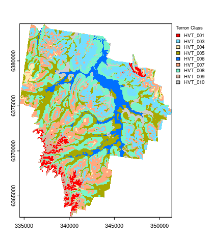
Apply model spatially
And finally, creating the map derived from the hv.C5 model using the terra::predict function. Note that the C5 model returned 0% producer’s accuracy for Terron classes 2, 11 and 12. These data account for only a small proportion of the data set, and/or, they may be similar to other existing Terron classes (based on the available predictive covariates). Consequently, they did not feature in the hv.C5 model and ultimately, the final map.
Another curiosity is that the model predictions also extends beyond the normal mapping boundary which does not mean much but one would want to remove these predictions as it causes the map product to look strange and potentially misleading. First we create a mask, msk and then use the mask function to blot out the areas where we do not need to have model predictions.
## Applying model spatially class prediction
map.C5.c <- terra::predict(object = hv.rasters, model = hv.C5, type = "class")

# mask [the C5 model extends to outside the mapping area]
msk <- terra::ifel(is.na(hv.rasters[[1]]), NA, 1)
map.C5.c.masked <- terra::mask(map.C5.c, msk, inverse = F)

# plot map
map.C5.c.masked <- as.factor(map.C5.c.masked)
# some classes were dropped out !!
levels(map.C5.c.masked)[[1]]

## HEX colors
area_colors <- c("#FF0000", "#73DFFF", "#FFEBAF", "#A8A800",  "#0070FF", "#FFA77F", "#7AF5CA", "#D7B09E", "#CCCCCC")

terra::plot(map.C5.c.masked, col = area_colors, plg = list(legend = c("HVT_001", "HVT_003", "HVT_004", "HVT_005", "HVT_006", "HVT_007", "HVT_008", "HVT_009", "HVT_010"), cex = 0.75, title = "Terron Class"))
References
Malone, B P, P Hughes, A B McBratney, and B Minsany. 2014. “A Model for the Identification of Terrons in the Lower Hunter Valley, Australia.” Geoderma Regional 1: 31–47.
Quinlan, J R. 1993. C4.5: Programs for Machine Learning. Morgan Kaufmann, San Mateo, California.