CODE:
Get the code used for this section here
Digital Land Suitability Assessment
- Introduction
- Coding an enterprise suitability assessment
- Getting started with some data
- First run of the suitability assessment
- Stepping it up some. Mapping enterprise suitability
Introduction
If we consider what digital soil assessment (DSA) is as described in Carre et al. (2007), an obvious candidate application is land suitability evaluation for a specified land use type, which Diepen et al. (1991) define as all methods to explain or predict the use potential of land.
Land evaluation in some sense has been in practice at least since the earliest known human civilizations. The shift to sedentary agriculture from nomadic lifestyles is at least indicative of a concerted effort of human investment to evaluate the potential and capacity of land and its soils to support some form of agriculture like cropping (Brevik and Hartemink 2010).
In the modern times there is a well-documented history of land evaluation practice and programs throughout the world, many of which are described in Mueller et al. (2010). Much of the current thinking around land evaluation for agriculture are well documented within the land evaluation guidelines prepared by the Food and Agriculture Organization of the United Nations (FAO) in 1976 (FAO 1976).
These guidelines have strongly influenced and continue to guide land evaluation projects throughout the world. The FAO framework is a crop specific LSA system with a 5-class ranking of suitability (FAO Land Suitability Classes) from 1: Highly Suitable to 5: Permanently Not Suitable. Given a suite of biophysical information from a site, each attribute is evaluated against some expert-defined thresholds for each suitability class. The final evaluation of suitability for the site is the one in which is most limiting.
Digital soil mapping complementing land evaluation assessment is being more regularly observed. Examples (in Australia) include (Kidd et al. 2012) in Tasmania and (Harms et al. 2015) in Queensland. Perhaps an obvious reason is that one can derive with digital soil and climate modeling, very attribute specific mapping which can be targeted specifically to a particular agricultural land use or even to a specific enterprise (Kidd et al. 2012).
In this section, an example is given of a DSA where enterprise suitability is assessed. The specific example is a digital land suitability assessment (LSA) for hazelnuts across an area of northern Tasmania, Australia (Meander Valley) which has been previously described in Malone et al. (2015).
Coding an enterprise suitability assessment
The example considered below is just to give an overview of how to perform a DSA in what could be considered as a relatively simple example.
Using the most-limiting factor approach of land suitability assessment, the procedure requires a pixel-by-pixel assessment of a number of input variables which have been expertly defined as being important for the establishment and growth of hazelnuts. Malone et al. (2015) describes the digital mapping processes that went into creating the input variables for this example.
The approach also assumes that the predicted maps of the input variables are also error free. The figure below shows an example of the input variable requirements and the suitability thresholds for hazelnuts. You will notice the biophysical variables include both soil and climatic variables, and the suitability classification has four levels of grading.
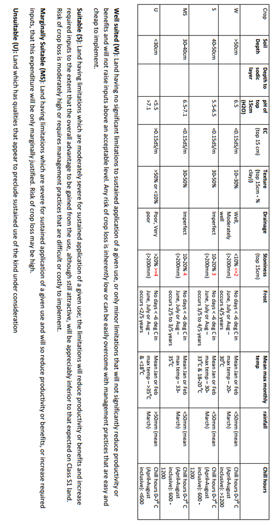
Probably the first thing to consider for enabling the DSA in this example is to codify the information above into an R function. It would look like something similar to the following script.
# HAZELNUT SUITABILITY ASSESSMENT FUNCTION
hazelnutSuits <- function(samp.matrix) {
out.matrix <- matrix(NA, nrow = nrow(samp.matrix), ncol = 10)  #ten selection variable for hazelnuts

# Chill Hours
out.matrix[which(samp.matrix[, 1] > 1200), 1] <- 1
out.matrix[which(samp.matrix[, 1] > 600 & samp.matrix[, 1] <= 1200), 1] <- 2
out.matrix[which(samp.matrix[, 1] <= 600), 1] <- 4

# Clay content
out.matrix[which(samp.matrix[, 2] > 10 & samp.matrix[, 2] <= 30), 2] <- 1
out.matrix[which(samp.matrix[, 2] > 30 & samp.matrix[, 2] <= 50), 2] <- 2
out.matrix[which(samp.matrix[, 2] > 50 | samp.matrix[, 2] <= 10), 2] <- 4

# Soil Drainage
out.matrix[which(samp.matrix[, 3] > 3.5), 3] <- 1
out.matrix[which(samp.matrix[, 3] <= 3.5 & samp.matrix[, 3] > 2.5), 3] <- 2
out.matrix[which(samp.matrix[, 3] <= 2.5 & samp.matrix[, 3] > 1.5), 3] <- 3
out.matrix[which(samp.matrix[, 3] <= 1.5), 3] <- 1

# EC (transformed variable)
out.matrix[which(samp.matrix[, 4] <= 0.15), 4] <- 1
out.matrix[which(samp.matrix[, 4] > 0.15), 4] <- 4

# Frost
out.matrix[which(samp.matrix[, 5] == 0), 5] <- 1
out.matrix[which(samp.matrix[, 5] != 0 & samp.matrix[, 6] >= 80), 5] <- 1
out.matrix[which(samp.matrix[, 5] != 0 & samp.matrix[, 6] < 80 & samp.matrix[,
6] >= 60), 5] <- 2
out.matrix[which(samp.matrix[, 5] != 0 & samp.matrix[, 6] < 60 & samp.matrix[,
6] >= 40), 5] <- 3
out.matrix[which(samp.matrix[, 5] != 0 & samp.matrix[, 6] < 40), 5] <- 3

# pH
out.matrix[which(samp.matrix[, 7] <= 6.5 & samp.matrix[, 7] >= 5.5), 6] <- 1
out.matrix[which(samp.matrix[, 7] > 6.5 & samp.matrix[, 7] <= 7.1), 6] <- 3
out.matrix[which(samp.matrix[, 7] < 5.5 | samp.matrix[, 7] > 7.1), 6] <- 4

# rainfall
out.matrix[which(samp.matrix[, 8] <= 50), 7] <- 1
out.matrix[which(samp.matrix[, 8] > 50), 7] <- 4

# soil depth
out.matrix[which(samp.matrix[, 9] == 0), 8] <- 1
out.matrix[which(samp.matrix[, 9] != 0 & samp.matrix[, 10] > 50), 8] <- 1
out.matrix[which(samp.matrix[, 9] != 0 & samp.matrix[, 10] <= 50 & samp.matrix[,
10] > 40), 8] <- 2
out.matrix[which(samp.matrix[, 9] != 0 & samp.matrix[, 10] <= 40 & samp.matrix[,
10] > 30), 8] <- 3
out.matrix[which(samp.matrix[, 9] != 0 & samp.matrix[, 10] <= 30), 8] <- 4

# temperature
out.matrix[which(samp.matrix[, 11] > 20 & samp.matrix[, 11] <= 30), 9] <- 1
out.matrix[which(samp.matrix[, 11] > 30 & samp.matrix[, 11] <= 33 | samp.matrix[,
11] <= 20 & samp.matrix[, 11] > 18), 9] <- 2
out.matrix[which(samp.matrix[, 11] > 33 & samp.matrix[, 11] <= 35), 9] <- 3
out.matrix[which(samp.matrix[, 11] > 35 | samp.matrix[, 11] <= 18), 9] <- 4

# rocks
out.matrix[which(samp.matrix[, 12] == 0), 10] <- 1
out.matrix[which(samp.matrix[, 12] != 0 & samp.matrix[, 13] <= 2), 10] <- 1
out.matrix[which(samp.matrix[, 12] != 0 & samp.matrix[, 13] == 3), 10] <- 2
out.matrix[which(samp.matrix[, 12] != 0 & samp.matrix[, 13] == 4), 10] <- 3
out.matrix[which(samp.matrix[, 12] != 0 & samp.matrix[, 13] > 4), 10] <- 4

return(out.matrix)
}
Essentially the function takes in a matrix of n number of rows by 13 columns. The number of columns is fixed as each coincides with one of the biophysical variables. There are some variables where there is relevant information contained in two columns. Soil depth is one of these variables. The reason is that soil depth is modeled via a two-stage process (as is exemplified in the section regarding two-stage modeling for DSM), such that a model is used to predict the presence/absence of a certain condition - which for soil depth is whether lithic contact is achieved less than 1.5 m from the soil surface - followed by a secondary model which predicts soil depth (where soil is expected to be less than 1.5m). Subsequently the secondary model is only invoked if there is a positive condition found for the first model.
The above R function provides a good example of the use of sub-setting and applying conditional queries within R applied in the introduction to R part of the course.
The function hazelnutSuits will return a new matrix with n rows and 10 columns (as there are 10 assessment criteria). The entries for each column and row will be the suitability assessment for each biophysical variable. It is then just a matter of determining what the maximum value is on each row in order to give an overall suitability valuation (as this is the most limiting factor approach). This can be achieved using the rowMaxs function from the matrixStats package.
Getting started with some data
Assuming there are digital soil and climate maps already created for use in the hazelnut land suitability assessment, it is relatively straightforward to run the LSA. Keep in mind that the creation of the biophysical variable maps were created via a number of means which included continuous attribute modeling, binomial and ordinal logistic regression, and a combination of both i.e. through the two-stage mapping process. So let’s get some sense of the LSA input variables we have to work with.
Sourcing of the input variables for this exercise comes from the ithirpackage.
# libraries
library(ithir)
library(terra)
library(matrixStats)

## Data for the exercise grids (lsa rasters from ithir package)
lsa.variables <- list.files(path = system.file("extdata/dsa/", package = "ithir"),
pattern = ".tif", full.names = TRUE)

# read them into R as SpatRaster objects
lsa.variables <- terra::rast(lsa.variables)
Take a look at the supplied data and perhaps perform your own checks and investigations. Some checks to get started include:
## Print out general raster metadata
lsa.variables

## class       : SpatRaster
## dimensions  : 1081, 1685, 13  (nrow, ncol, nlyr)
## resolution  : 30, 30  (x, y)
## extent      : 452246.4, 502796.4, 5387368, 5419798  (xmin, xmax, ymin, ymax)
## coord. ref. :


# LSA names and class
names(lsa.variables)

##  [1] "X1_chill_HAZEL_FINAL_meandertif"
##  [2] "X10_rocks_binaryClass_meandertif"
##  [3] "X11_rocks_ordinalClass_meandertif"
##  [4] "X2_clay_FINAL_meandertif"
##  [5] "X3_drain_FINAL_meandertif"
##  [6] "X4_EC_cubist_meandertif"
##  [7] "X5_Frost_HAZEL_binaryClass_meandertif"
##  [8] "X5_Frost_HAZEL_FINAL_meandertif"
##  [9] "X6_pH_FINAL_meandertif"
## [10] "X7_rain_HAZEL_FINAL_meandertif"
## [11] "X8_soilDepth_binaryClass_meandertif"
## [12] "X8_soilDepth_FINAL_meandertif"
## [13] "X9_temp_HAZEL_FINAL_meandertif"

class(lsa.variables)

## [1] "SpatRaster"
## attr(,"package")
## [1] "terra"

# Raster stack dimensions: layers, row num, col num
terra::nlyr(lsa.variables)

## [1] 13

terra::nrow(lsa.variables)

## [1] 1081

terra::ncol(lsa.variables)

## [1] 1685

# Raster resolution
terra::res(lsa.variables)

## [1] 30 30
First run of the suitability assessment
There are 13 rasters of data, which you will note coincide with the inputs required for the hazelnutSuits function. Now all that is required is to go pixel by pixel and apply the LSA function. In R the implementation may take the following form:
## EXAMPLE ON ONE ROW OF A RASTER Retrieve values of from all rasters for a
## given row Here it is the 100th row of the raster
# get all soil and climate data for selected row
cov.Frame <- lsa.variables[100, ]
nrow(cov.Frame)

## [1] 1685

# Remove the pixels where there is NA or no data present
sub.frame <- cov.Frame[which(complete.cases(cov.Frame)), ]
nrow(sub.frame)

## [1] 120

names(sub.frame)

##  [1] "X1_chill_HAZEL_FINAL_meandertif"
##  [2] "X10_rocks_binaryClass_meandertif"
##  [3] "X11_rocks_ordinalClass_meandertif"
##  [4] "X2_clay_FINAL_meandertif"
##  [5] "X3_drain_FINAL_meandertif"
##  [6] "X4_EC_cubist_meandertif"
##  [7] "X5_Frost_HAZEL_binaryClass_meandertif"
##  [8] "X5_Frost_HAZEL_FINAL_meandertif"
##  [9] "X6_pH_FINAL_meandertif"
## [10] "X7_rain_HAZEL_FINAL_meandertif"
## [11] "X8_soilDepth_binaryClass_meandertif"
## [12] "X8_soilDepth_FINAL_meandertif"
## [13] "X9_temp_HAZEL_FINAL_meandertif"

# run hazelnutSuits function
# first, order the data frame so columns match to assessment criteria in the function
sub.frame <- sub.frame[, c(1, 4:13, 2, 3)]
hazel.lsa <- hazelnutSuits(sub.frame)

# Assess for suitability
matrixStats::rowMaxs(hazel.lsa)

##   [1] 2 2 2 2 4 4 4 4 4 4 4 4 3 4 4 4 4 4 4 4 4 4 4 4 4 4 4 4 4 4 4 4 4 4 4 4 4
##  [38] 4 4 4 4 4 4 4 4 4 4 4 4 4 4 4 4 4 4 4 4 4 4 4 4 4 4 4 4 4 4 4 4 4 4 4 4 4
##  [75] 4 4 4 4 4 4 4 4 4 4 4 4 4 4 4 4 4 4 4 4 4 4 4 4 4 2 2 2 2 2 2 2 2 2 2 2 2
## [112] 2 2 4 4 4 4 4 4 4
The above script has just performed the hazelnut LSA upon the entire selected row of the input variable rasters where there was available data after excluding all the NA values.
Stepping it up some. Mapping enterprise suitability
To do the LSA for the entire mapping extent we could effectively run the script above for each row of the input rasters. Naturally, this would take an age to do manually, so it might be more appropriate to use the script above inside a for loop where the row index changes for each loop. Refer to previous exercises on the use of for loops.
Alternatively, the custom hazelnutSuits function could be used as an input argument for the terra package app function.
Given the available options, we will demonstrate the mapping process using the looping approach. While it may be computationally slower, it imprints the concept of applying the LSA spatially.
From the above script and resulting output, we essentially returned a vector of integers. We effectively lost all links to the fact that the inputs and resulting outputs are spatial data. Subsequently there is a need to link the suitability assessment back to the mapping.
Fortunately we know the column positions of the instances where there was the full suite of input data. So once we have set up a raster object to which data can be written to (which has the same raster properties of the input data), it is just a matter of placing the LSA outputs into the row and column positions as those of the input data.
A full example is given below, but for the present purpose, the LSA output data placement into a raster would look something like the following:
# A one column matrix with number of rows equal to number of columns in raster inputs
a.matrix<- matrix(NA, nrow=nrow(cov.Frame), ncol= 1)

#Place LSA outputs into correct row positions
a.matrix[which(complete.cases(cov.Frame)),1]<- matrixStats::rowMaxs(hazel.lsa)

#Write LSA outputs to raster object (here the 100th row)
LSA.raster<- terra::writeValues(x = LSA.raster,v = a.matrix[,1], start = 100 nrows = 1)
Naturally the above few lines of script would also be embedded into the looping process as described above. Below is an example of putting all these operations together to ultimately produce a map of the suitability assessment.
To add a slight layer of complexity, we may also want to produce maps of the suitability assessment for each of the input variables. This helps in determining which factors are causing the greatest limitations and where they occur. First, we need to create a number of rasters to which we can write the outputs of the LSA to.
## Create a suite of rasters with same raster properties is LSA input variables

# general file path where raster are to be saved
loc <- "/home/tempfiles/"

# Overall suitability classification
LSA.raster <- rast(lsa.variables[[1]])
# Write outputs of LSA directly to file
terra::writeStart(LSA.raster, filename = paste0(loc, "meander_MLcat.tif"), datatype = "INT2S", overwrite = TRUE)

# Individual LSA input suitability rasters
mlf1 <- rast(lsa.variables[[1]])
mlf2 <- rast(lsa.variables[[1]])
mlf3 <- rast(lsa.variables[[1]])
mlf4 <- rast(lsa.variables[[1]])
mlf5 <- rast(lsa.variables[[1]])
mlf6 <- rast(lsa.variables[[1]])
mlf7 <- rast(lsa.variables[[1]])
mlf8 <- rast(lsa.variables[[1]])
mlf9 <- rast(lsa.variables[[1]])
mlf10 <- rast(lsa.variables[[1]])

# Also write individual LSA outputs directly to file.
terra::writeStart(mlf1, filename = paste0(loc, "meander_Haz_mlf1_CAT.tif"), datatype = "INT2S", overwrite = TRUE)
terra::writeStart(mlf2, filename = paste0(loc, "meander_Haz_mlf2_CAT.tif"), datatype = "INT2S", overwrite = TRUE)
terra::writeStart(mlf3, filename = paste0(loc, "meander_Haz_mlf3_CAT.tif"), datatype = "INT2S", overwrite = TRUE)
terra::writeStart(mlf4, filename = paste0(loc, "meander_Haz_mlf4_CAT.tif"), datatype = "INT2S", overwrite = TRUE)
terra::writeStart(mlf5, filename = paste0(loc, "meander_Haz_mlf5_CAT.tif"), datatype = "INT2S", overwrite = TRUE)
terra::writeStart(mlf6, filename = paste0(loc, "meander_Haz_mlf6_CAT.tif"), datatype = "INT2S", overwrite = TRUE)
terra::writeStart(mlf7, filename = paste0(loc, "meander_Haz_mlf7_CAT.tif"), datatype = "INT2S", overwrite = TRUE)
terra::writeStart(mlf8, filename = paste0(loc, "meander_Haz_mlf8_CAT.tif"), datatype = "INT2S", overwrite = TRUE)
terra::writeStart(mlf9, filename = paste0(loc, "meander_Haz_mlf9_CAT.tif"), datatype = "INT2S", overwrite = TRUE)
terra::writeStart(mlf10, filename = paste0(loc, "meander_Haz_mlf10_CAT.tif"), datatype = "INT2S", overwrite = TRUE)
Now we can implement the for loop procedure and do the LSA for the entire mapping extent.
# Run the suitability model row by row:
for (i in 1:nrow(LSA.raster)) {
  # get raster values
  cov.Frame <- lsa.variables[i, ]
  # get the complete cases
  sub.frame <- cov.Frame[which(complete.cases(cov.Frame)), ]

  # re-order the data frame
  sub.frame <- sub.frame[, c(1, 4:13, 2, 3)]

  # Run hazelnut LSA function
  t1 <- hazelnutSuits(sub.frame)

  # Save results to raster
  a.matrix <- matrix(NA, nrow = nrow(cov.Frame), ncol = 1)
  a.matrix[which(complete.cases(cov.Frame)), 1] <- matrixStats::rowMaxs(t1)
  terra::writeValues(LSA.raster, a.matrix[, 1], start = i, nrows = 1)

  # Also save the single input variable assessment outputs
  mlf.out <- matrix(NA, nrow = nrow(cov.Frame), ncol = 10)
  mlf.out[which(complete.cases(cov.Frame)), 1] <- t1[, 1]
  mlf.out[which(complete.cases(cov.Frame)), 2] <- t1[, 2]
  mlf.out[which(complete.cases(cov.Frame)), 3] <- t1[, 3]
  mlf.out[which(complete.cases(cov.Frame)), 4] <- t1[, 4]
  mlf.out[which(complete.cases(cov.Frame)), 5] <- t1[, 5]
  mlf.out[which(complete.cases(cov.Frame)), 6] <- t1[, 6]
  mlf.out[which(complete.cases(cov.Frame)), 7] <- t1[, 7]
  mlf.out[which(complete.cases(cov.Frame)), 8] <- t1[, 8]
  mlf.out[which(complete.cases(cov.Frame)), 9] <- t1[, 9]
  mlf.out[which(complete.cases(cov.Frame)), 10] <- t1[, 10]
  terra::writeValues(mlf1, mlf.out[, 1], start = i, nrows = 1)
  terra::writeValues(mlf2, mlf.out[, 2], start = i, nrows = 1)
  terra::writeValues(mlf3, mlf.out[, 3], start = i, nrows = 1)
  terra::writeValues(mlf4, mlf.out[, 4], start = i, nrows = 1)
  terra::writeValues(mlf5, mlf.out[, 5], start = i, nrows = 1)
  terra::writeValues(mlf6, mlf.out[, 6], start = i, nrows = 1)
  terra::writeValues(mlf7, mlf.out[, 7], start = i, nrows = 1)
  terra::writeValues(mlf8, mlf.out[, 8], start = i, nrows = 1)
  terra::writeValues(mlf9, mlf.out[, 9], start = i, nrows = 1)
  terra::writeValues(mlf10, mlf.out[, 10], start = i, nrows = 1)
  print((nrow(LSA.raster)) - i)
  }  #END OF LOOP

# complete writing rasters to file
LSA.raster <- writeStop(LSA.raster)
mlf1 <- writeStop(mlf1)
mlf2 <- writeStop(mlf2)
mlf3 <- writeStop(mlf3)
mlf4 <- writeStop(mlf4)
mlf5 <- writeStop(mlf5)
mlf6 <- writeStop(mlf6)
mlf7 <- writeStop(mlf7)
mlf8 <- writeStop(mlf8)
mlf9 <- writeStop(mlf9)
mlf10 <- writeStop(mlf10)
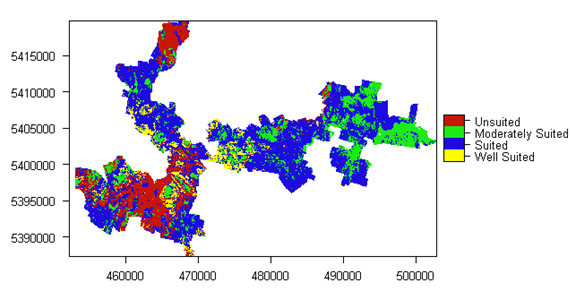
As you may encounter, the above script can take quite a while to complete, but ultimately you should be able to produce a number of mapping products. The figure below shows the map of the overall suitability classification and the script to produce it is below.
names(LSA.raster) <- "Hazelnut suitability"
LSA.raster <- as.factor(LSA.raster)
levels(LSA.raster) = data.frame(value = 1:4, desc = c("Well Suited", "Suited", "Moderately Suited", "Unsuited"))
area_colors <- c("#FFFF00", "#1D0BE0", "#1CEB15", "#C91601")
plot(LSA.raster, col = area_colors, plg = list(loc = "bottomright"))
Similarly the above plotting procedure can be repeated to look at single input variable limitations too.
The approaches detailed in this chapter are described in greater detail in Malone et al. (2015) within the context of taking account of uncertainties within LSA. Taking account of the input variable uncertainties adds an additional level of complexity to what was achieved above, but is an important consideration nonetheless, as the resulting outputs can be assessed for reliability in an objective manner.
References
Brevik, Eric C., and Alfred E. Hartemink. 2010. “Early Soil Knowledge and the Birth and Development of Soil Science.” Catena 83 (1): 23–33. https://doi.org/http://dx.doi.org/10.1016/j.catena.2010.06.011.
Carre, F., Alex B. McBratney, Thomas Mayr, and Luca Montanarella. 2007. “Digital Soil Assessments: Beyond DSM.” Geoderma 142 (1-2): 69–79. https://doi.org/http://dx.doi.org/10.1016/j.geoderma.2007.08.015.
Diepen, C. A. van, H. van Keulen, J. Wolf, and J. A. A. Berkhout. 1991. “Land Evaluation: From Intuition to Quantification.” In Advances in Soil Science, edited by B. A. Stewart, 15:139–204. Advances in Soil Science. Springer New York. https://doi.org/10.1007/978-1-4612-3030-4_4.
FAO. 1976. A Framework for Land Evaluation. Soils Bulletin 32. Rome: Food; Agriculture Organisation of the United Nations.
Harms, B., D. Brough, S. Philip, R. Bartley, D. Clifford, M. Thomas, R. Willis, and L. Gregory. 2015. “Digital Soil Assessment for Regional Agricultural Land Evaluation.” Global Food Security 5: 25–36. https://doi.org/http://dx.doi.org/10.1016/j.gfs.2015.04.001.
Kidd, Darren B., M. A. Webb, C. J. Grose, R. M. Moreton, Brendan P. Malone, Alex B. McBratney, Budiman Minasny, Raphael Viscarra-Rossel, L. A. Sparrow, and R. Smith. 2012. “Digital Soil Assessment: Guiding Irrigation Expansion in Tasmania, Australia.” Edited by Budiman Minasny, Brendan P. Malone, and Alex B. McBratney. Boca Raton: CRC.
Kidd, Darren, Mathew Webb, Brendan Malone, Budiman Minasny, and Alex McBratney. 2015. “Digital Soil Assessment of Agricultural Suitability, Versatility and Capital in Tasmania, Australia.” Geoderma Regional 6: 7–21. https://doi.org/http://dx.doi.org/10.1016/j.geodrs.2015.08.005.
Malone, Brendan P., Darren B. Kidd, Budiman Minasny, and Alex B. McBratney. 2015. “Taking Account of Uncertainties in Digital Land Suitability Assessment.” PeerJ, 3:e1366.
McBratney, Alex B., Budiman Minasny, Ischani Wheeler, Brendan P. Malone, and David Van Der Linden. 2012. “Frameworks for Digital Soil Assessment.” Edited by Budiman Minasny, Brendan P. Malone, and Alex B. McBratney. London, UK: CRC Press.
Mueller, Lothar, Uwe Schindler, Wilfried Mirschel, T.Graham Shepherd, BruceC. Ball, Katharina Helming, Jutta Rogasik, Frank Eulenstein, and Hubert Wiggering. 2010. “Assessing the Productivity Function of Soils. A Review.” Agronomy for Sustainable Development 30 (3): 601–14. https://doi.org/10.1051/agro/2009057.